ODEs (Ordinary Differential Equations)_Справочник по пакету Mathematica

ODEs (Ordinary Differential Equations)

Справочник по пакету Mathematica

ODEs (Ordinary Differential Equations)

In the Mathematica examples below, boldface type is Input, regular type is Output.

y''=3-y

Some differential equations permit general, analytic solutions:


  DSolve[ y''[t]==3-y[t], y[t], t ]

    {{y[t] -> 3 + C[2]*Cos[t] - C[1]*Sin[t]}}

y'=sin(y), y(1)=4.2

Numerical solutions to ODEs --- Initial Value Problems), where initial values for y and y', etc. are given --- are in the form of "interpolating functions";


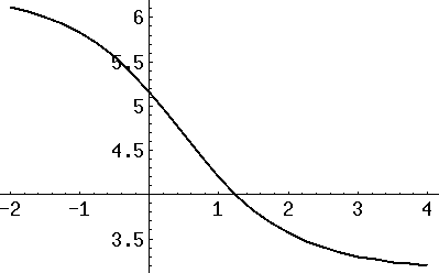
  soln = NDSolve[ {y'[t] == Sin[y[t]], y[1]==4.2}, y, {t, -2, 4} ]

    {{y -> InterpolatingFunction[{-2., 4.},  ... }}

How do you use ``InterpolatingFunction''? It can give you specific numerical values (approximations, of course) and graphs. Using soln[[1]] from the solution above,


   Table[ {x, y[x], y'[x]} /. soln[[1]], {x,-1,3,0.5} ] // TableForm

         - 1      5.82839   -0.439294
         - 0.5    5.55424   -0.666085
           0.     5.16022   -0.901381
           0.5    4.67599   -0.999343
           1.     4.2       -0.87127
           1.5    3.82336   -0.630159
           2.     3.56544   -0.411271
           2.5    3.40112   -0.256627


   Plot[ y[x] /. soln[[1]], {x,-2,4} ];

Solving xy'+2y=sin(x) numerically

The following example shows how to use Mathematica to display a vector field and a specific trajectory, for a differential equation and starting value (IVP). The PlotField function requires that the standard package "Graphics`PlotField`" be loaded. All other comands are basic Mathematica functions described in the book Mathematica, a System for doing Mathematics by Computer (Wolfram).


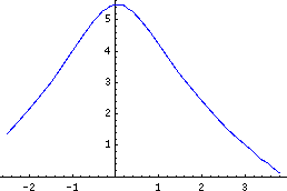
     gensoln = DSolve[ x y'[x] + 2y[x] == Sin[x], y[x], x]

               C[1]   -(x Cos[x]) + Sin[x] 
     {{y[x] -> ---- + --------------------}}
		 2              2
                x              x


     onesoln = gensoln[[1]] /. C[1]->1.3;
     y[x_] = y[x] /. onesoln

     trajectory = Plot[ y[x], {x,1,10}, PlotRange->All,
			PlotStyle->{Hue[0.67]}];

     
     1.3   -(x Cos[x]) + Sin[x]
     --- + --------------------
      2              2
     x              x



     Needs["Graphics`PlotField`"];
     field = PlotVectorField[ {1, (Sin[x]-2y)/x},
		{x, 0.1, 10}, {y, -1, 2}];


     
     Show[ field, trajectory ];

Numerical solution of x(t) y'(t) +2y(t) = sin(x(t))

The vector field specified by a differential equation can be represented graphically using a standard package -- a set of special commands which can be loaded with the following command:


     Needs["Graphics`PlotField`"];

The differential equation x(t) y(t)'+2y(t) = sin(x(t)) can be set up as a set of two equations in terms of the independent parameter t, one for x'(t) and one for y'(t):


     eq1  =  x'[t] == y[t];
     eq2  =  y'[t] == (Sin[x[t]]-2y[t])/x[t];

Here's how to show a representation of the associated field. Let's show it for values of 1<x<5 and -1<y<2:


     field  =  PlotVectorField[ {y, Sin[x]-2y)/x}, {x,1,5, 0.25}, {y,-1,2, 0.2}];

Now, one particular solution, obeying this differential equation plus the initial conditions x(0)=3 and y(0)=1, can be displayed using ParametricPlot. First solve the ODE numerically. We must give an explicit range for the parameter t; the range -0.5<t<15 gives a nice solution and picture. (Hue 0.67 is blue.)


     nsoln = NDSolve[ {eq1, eq2, x[0]==3, y[0]==1}, {x,y}, {t, -0.5, 15}];
     trajectory = ParametricPlot[ {x[t], y[t]} /. nsoln[[1]], {t, -0.5, 15},
			PlotRange->All,   PlotStyle->{Hue[0.67]}];

The two graphics above can be shown together, using Show. Note that the specific solution for the given initial conditions (trajectory) fits with the general solution (field).


     Show[trajectory, field];

Numerical solution of (1+x²)y'+4xy = (1+x²)^-2

In this case, the differential equation (1+x²)y'+4xy = (1+x²)^-2 can be set up as the following set of two equations;


     eq1  =  x'[t] == y[t];
     eq2  =  y'[t] == (1/(1+x[t]^2)^2-4x[t] y[t])/(1+x[t]^2)

Here's a nice picture of the field defined by these equations:


     field  =  PlotVectorField[ {y, (1/(1+x^2)^2-4x y)/(1+x^2)},
     			{x,-4,4, 0.5}, {y,0,7, 0.5}];

Solving for initial conditions, say, x(0)=3 and y(0)=1, and displaying the trajectory {x(t), y(t)} parametrically in blue,


     nsoln = NDSolve[ {eq1, eq2, x[0]==3, y[0]==1}, {x,y}, {t, -2, 2}];
     trajectory = ParametricPlot[ {x[t], y[t]} /. nsoln[[1]], {t, -2, 2},
			PlotRange->All,   PlotStyle->{Hue[0.67]}];

Show the general field and the specific solution together:


     Show[trajectory, field];

Назад