This paper addresses the well-known classification task of data mining, where the objective is to predict the class which an example belongs to. Discovered knowledge is expressed in the form of high-level, easy-to-interpret classification rules. In order to discover classification rules, we propose a hybrid decision tree/genetic algorithm method. The central idea of this hybrid method involves the concept of small disjuncts in data mining, as follows. In essence, a set of classification rules can be regarded as a logical disjunction of rules, so that each rule can be regarded as a disjunct. A small disjunct is a rule covering a small number of examples. Due to their nature, small disjuncts are error prone. However, although each small disjunct covers just a few examples, the set of all small disjuncts can cover a large number of examples, so that it is important to develop new approaches to cope with the problem of small disjuncts. In our hybrid approach, we have developed two genetic algorithms (GA) specifically designed for discovering rules covering examples belonging to small disjuncts, whereas a conventional decision tree algorithm is used to produce rules covering examples belonging to large disjuncts. We present results evaluating the performance of the hybrid method in 22 real-world data sets.
This paper addresses the well-known classification task of data mining [16]. In this task, the discovered knowledge is often expressed as a set of rules of the form:
IF <conditions> THEN <prediction (class)>.
This knowledge representation has the advantage of being intuitively comprehensible for the user, and it is the kind of knowledge representation used in this paper. From a logical viewpoint, typically the discovered rules are expressed in disjunctive normal form, where each rule represents a disjunct and each rule condition represents a conjunct. In this context, a small disjunct can be defined as a rule which covers a small number of training examples [17].
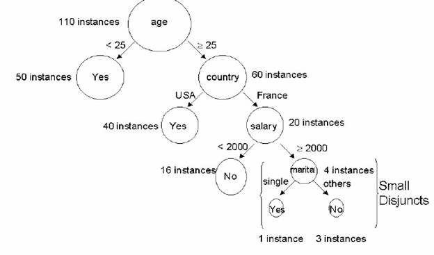
The concept of small disjunct is illustrated in Fig 1. This figure shows a part of a decision tree induced from the Adult data set, one of the data sets used in our experiments (section 4). In this figure we indicate, beside each tree node, the number of examples belonging to that node. Hence, the two leaf nodes at the right bottom can be considered small disjuncts, since they have just one and three examples (instances).
Fig 1: Example of a small disjunct in a decision tree induced from the Adult data set
The vast majority of rule induction algorithms have a bias that favors the discovery of large disjuncts, rather than small disjuncts. This preference is due to the belief that it is better to capture generalizations rather than specializations in the training set, since the latter are unlikely to be valid in the test set [10].
Note that classifying examples belonging to large disjuncts is relatively easy. For instance, in Fig 1, consider the leaf node predicting class "Yes" for examples having Age < 25, at the left top of the figure. Presumably, we can be confident about this prediction, since it is based on 50 examples. By contrast, in the case of small disjuncts, we have a small number of examples, and so the prediction is much less reliable. The challenge is to accurately predict the class of small- disjunct examples.
At first glance, perhaps one could ignore small disjuncts, since they tend to be error prone and seem to have a small impact on predictive accuracy. However, small disjuncts are actually quite important in data mining and should not be ignored. The main reason is that, even though each small disjunct covers a small number of examples, the set of all small disjuncts can cover a large number of examples. For instance [10] reports a real-world application where small disjuncts cover roughly 50% of the training examples. In such cases we need to discover accurate small-disjunct rules in order to achieve a good classification accuracy rate.
Our approach for coping with small disjuncts consists of a hybrid decisiontree/ genetic algorithm method, as will be described in section 2. The basic idea is that examples belonging to large disjuncts are classified by rules produced by a decision-tree algorithm, while examples belonging to small disjuncts are classified by a genetic algorithm (GA) designed for discovering small-disjunct rules. This approach is justified by the fact that GAs tend to cope better with attribute interaction than conventional greedy decision-tree/rule induction algorithms (see section 2), and attribute interaction can be considered one of the main causes of the problem of small disjuncts [11], [25], [26].
The rest of this paper is organized as follows. Section 2 describes the main characteristics of our hybrid decision tree/genetic algorithm method for coping with small disjuncts. This section assumes that the reader is familiar with the basic ideas of decision trees and genetic algorithms. Section 3 describes two GAs specifically designed for discovering small-disjunct rules, in order to realize the GA component of our hybrid method. Section 4 reports the results of extensive experiments evaluating the performance of our hybrid method, with respect to predictive accuracy, across 22 data sets. The experiments also compare the performance of the hybrid method with the performance of two versions of a decision tree algorithm. Section 5 discusses related work. Finally, section 6 concludes the paper.
In this section we describe the main characteristics of our method for coping with the problem of small disjuncts. This is a hybrid method that combines decision trees and genetic algorithms [5], [6], [3], [4]. The basic idea is to use a decision-tree algorithm to classify examples belonging to large disjuncts and use a genetic algorithm to discover rules classifying examples belonging to small disjuncts.
The method discovers rules in two training phases. In the first phase it runs C4.5, a well-known decision tree induction algorithm [24]. The induced, pruned tree is transformed into a set of rules. As mentioned in the Introduction, this rule set can be thought of as expressed in disjunctive normal form, so that each rule corresponds to a disjunct. Each rule is considered either as a small disjunct or as a “large” (non-small) disjunct, depending on whether or not its coverage (the number of examples covered by the rule) is smaller than or equal to a given threshold. The second phase consists of using a genetic algorithm to discover rules covering the examples belonging to small disjuncts. This two-phase process is summarized in Fig 2.
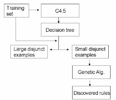
Fig 2: Overview of our hybrid decision tree/GA method for discovering small-disjunct rules
After the GA run is over, examples in the test set are classified as follows. Each example to be classified is pushed down the decision tree until it reaches a leaf node, as usual. If the leaf node is a large disjunct, the example is assigned the class predicted by that leaf node. Otherwise - i.e., the leaf node is a small disjunct - the example is assigned the class of one of the small-disjunct rules discovered by the GA.
The basic idea of the method – i.e., using a decision tree to classify largedisjunct examples and using a GA to classify small-disjunct examples – can be justified as follows.
Decision-tree algorithms have a bias towards generality that is well suited for large disjuncts, but not for small disjuncts. On the other hand, genetic algorithms are robust, flexible search algorithms which tend to cope with attribute interaction better than most rule induction algorithms [13], [9], [11], [12]. The reasons why GAs – and evolutionary algorithms in general – tend to cope well with attribute interaction have to do with the global-search nature of GAs, as follows. First, GAs work with a population of candidate solutions (individuals). Second, in GAs a candidate solution is evaluated as a whole by the fitness function. These characteristics are in contrast with most greedy rule induction algorithms, which work with a single candidate solution at a time and typically evaluate a partial candidate solution, based on local information only. Third, GAs use probabilistic operators that make them less prone to get trapped into local minima in the search space. Empirical evidence that in general GAs cope with attribute interaction better than greedy rule induction algorithms can be found in [9], [15], [22].
Intuitively, the ability of GAs to cope with attribute interaction makes them a potentially useful solution for the problem of small disjuncts, since, as mentioned in the Introduction, attribute interactions can be considered one of the causes of small disjuncts [11], [25], [26].
On the other hand, GAs also have some disadvantages for rule discovery, of course. First, in general they are considerably slower than greedy rule induction algorithms. Second, conventional genetic operators such as crossover and mutation are usually “blind”, in the sense that they are applied without directly trying to optimize the quality of the new candidate solution that they propose. (The optimization of candidate solutions is directly taken into account by the fitness function and the selection method, of course.)
Concerning the above first problem, although the hybrid decision tree/GA method proposed here is slower than a pure decision tree method, the increase in computational time turned out not to be a serious problem in our experiments, as will be seen later. Concerning the above second problem, it is a major problem in the application of GAs to data mining. The general solution, which was indeed the approach followed in the development of the GAs described in this paper, is to extend the GA with “genetic” operators that incorporate task-dependent knowledge – i.e., knowledge about the data mining task being solved – as will be seen later.
So far we have described our hybrid decision tree/GA method in a high level of abstraction, without going into details of the decision tree or the GA part of the method. The decision tree part of the method is a conventional decision tree algorithm, so it is not discussed here. On the other hand, the GA part of the method needs to be discussed in detail here, since it was especially developed for discovering small disjunct rules. Actually, we have developed two GAs for discovering small disjunct rules, as discussed in the next section.
Although the two GAs described in this section have some major differences, they also share some basic characteristics, such as the same structure of an individual’s genome and the same fitness function. This is due to the fact that in both GAs an individual represents essentially the same kind of candidate solution, namely a candidate small-disjunct rule. Hence, we first describe these common characteristics, and in the next two subsections we describe the characteristics that are specific to each of the two GAs.
Let us start with the structure of an individual’s genome. In both GAs an individual represents the antecedent (the IF part) of a single classification rule. This rule is a small-disjunct rule, in the sense that it is induced from a set of examples that has been considered a small disjunct, as explained in section 2.
The consequent (THEN part) of the rule, which specifies the predicted class, is not represented in the genome. The methods used to determine the consequent of the rule are different in the two GAs described in this paper, so these methods will be described later. In both GAs, the genome of an individual consists of a conjunction of conditions composing a given rule antecedent. Each condition is an attributevalue pair, as shown in Fig 3.

Fig 3: Structure of the genome of an individual.
In Fig 3 Ai denotes the i-th attribute and Opi denotes a logical/relational operator comparing Ai with one or more values Vij belonging to the domain of Ai, as follows. If attribute Ai is categorical (nominal), the operator Opi is “ in” , which will produce rule conditions such as “ Ai in {Vi1,...,Vik}” , where {Vi1,...,Vik} is a subset of the values of the domain of Ai. By contrast, if Ai is continuous (realvalued), the operator Opi is either “ d“ or “ >“ , which will produce rule conditions such as “ Ai d Vij” , where Vij is a value belonging to the domain of Ai. Each condition in the genome is associated with a flag, called the active bit Bi, which takes on the value 1 or 0 to indicate whether or not, respectively, the i-th condition occurs in the decoded rule antecedent. This allows the GA to use a fixed-length genome (for the sake of simplicity) to represent a variable-length rule antecedent.
Let us now turn to the fitness function – i.e., to the function used to evaluate the quality of the candidate small-disjunct rule represented by an individual. In both GAs described in this paper, the fitness function is given by the formula:
Fitness = (TP / (TP + FN)) * (TN / (FP + TN))
where TP, FN, TN and FP – standing for the number of true positives, false negatives, true negatives and false positives – are well-known variables often used to evaluate the performance of classification rules – see e.g. [16]. In the above formula the term (TP / (TP + FN)) is usually called sensitivity (Se) or true positive rate, whereas the term (TN / (FP + TN)) is usually called specificity (Sp) or true negative rate. These two terms are multiplied to foster the GA to discover rules having both high Se and high Sp. This is important because it would be relatively simple (but undesirable) to maximize one of these two terms at the expense of reducing the value of the other. It is now time to explain the most important difference between the two GAs for discovering small-disjunct rules described in this paper. This difference is the way the training set of each GA is formed. Recall, from section 2, that small disjuncts are identified as decision tree leaf nodes having a small number of examples. This gives us at least two possibilities to form a training set containing 7 small-disjunct examples. The first approach consists of associating the examples of each leaf node defining a small disjunct with a training set. This approach leds to the formation of d training sets, where d is the number of small disjuncts. This approach is illustrated in Fig 4(a). Note that each of these d training sets will be small, containing just a few examples. In this approach the GA will have to be run d times, each time with a different (but always small) training set, corresponding to a different small disjunct. The second approach consists of grouping all the examples belonging to all the leaf nodes considered small disjuncts into a single training set, called the “ second training set” (to distinguish it from the original training set used to build the decision tree). This approach is illustrated in Fig 4(b). Obviously, this second training set will be relatively large – i.e., it will contain many more examples than any of the small training sets formed in the first approach. Now, in principle the GA can be run just once to discover rules classifying all the examples in the second training set, as long as we use some kind of niching to ensure that the GA discovers a set of rules (rather than a single rule), as will be seen later.

Fig 4: Two approaches for creating training sets with small-disjunct examples
We stress that the two approaches illustrated in Fig 4 differ mainly with respect to the size of the training set given to the GA, and that this difference has profound consequences for the design of the two GAs described in the next two subsections. These two GAs are hereafter called GA-Small and GA-Large-SN.
The name GA-Small was chosen to emphasize that the GA in question discovers rules from a small training set, following the approach illustrated in Fig 4(a). The name GA-Large-SN was chosen to emphasize that the GA in question discovers rules from a relatively large training set, following the approach illustrated in Fig 4(b), and uses a Sequential Niching (SN) method.
Recall that an individual represents the antecedent (IF part) of a small-disjunct rule. For a given GA-Small run, the genome of an individual consists of n genes (conditions), where n = m - k, and where m is the total number of predictor attributes in the dataset and k is the number of ancestor nodes of the decision tree leaf node identifying the small disjunct in question. Hence, the genome of a GASmall individual contains only the attributes that were not used to label any ancestor of the leaf node defining that small disjunct. Note that in general the attributes used to label any ancestor of that leaf node are not useful for composing small-disjunct rules, since they are not good at discriminating the classes of examples in that leaf node.
The consequent (THEN part) of the rule, specifying the class predicted by that rule, is fixed for a given GA-Small run. Therefore, all individuals have the same rule consequent during all that run.
GA-Small uses conventional tournament selection, with tournament size of two [2], [21]. It also uses standard one-point crossover with crossover probability of 80%, and mutation probability of 1%. Furthermore, it uses elitism with an elitist factor of 1 – i.e. the best individual of each generation is passed unaltered into the next generation.
In addition to the above standard genetic operators, GA-Small also includes an operator especially designed for simplifying candidate rules. The basic idea of this rule-pruning operator is to remove several conditions from a rule to make it shorter. This operator is applied to every individual of the population, right after the individual is formed.
Unlike the usually simple operators of conventional GAs, GA-Small’ s rulepruning operator is an elaborate procedure based on information theory [8]. Hence, it can be regarded as a way of incorporating a classification-related heuristic into a GA for classification-rule discovery. In essence, this rule-pruning operator works as follows [3].
First of all, it computes the information gain of each of the n rule conditions (genes) in the genome of the individual – see below. Then the procedure iteratively tries to remove one condition at a time from the rule. The smaller the information gain of the condition, the earlier its removal is considered and the higher the probability that it will be actually removed from the rule.
More precisely, in the first iteration the condition with the smallest information gain is considered. This condition is kept in the rule (i.e. its active bit is set to 1) with probability equal to its normalized information gain (in the range 0..1), and is removed from the rule (i.e. its active bit is set to 0) with the complement of that probability. Next the condition with the second smallest information gain is considered. Again, this condition is kept in the rule with probability equal to its information gain, and is removed from the rule with the complement of that probability. This iterative process is performed while the number of conditions occurring in the rule is greater than the minimum number of rule conditions and the iteration number is smaller than or equal to the number of genes (maximum number of rule conditions) n.
The information gain of each rule condition condi of the form <Ai Opi Vij> is computed as follows [8], [24]:
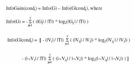
where G is the goal (class) attribute, c is the number of classes (values of G), |Gj| is the number of training examples having the j-th value of G, |T| is the total number of training examples, |Vi| is the number of training examples satisfying the condition <Ai Opi Vij>, |Vij| is the number of training examples that both satisfy the condition <Ai Opi Vij> and have the j-th value of G, |oVi| is the number of training examples that do not satisfy the condition <Ai Opi Vij>, and |oVij| is the number of training examples that do not satisfy <Ai Opi Vij> and have the j-th value of G. The use of the above rule-pruning procedure combines the stochastic nature of GAs, which is partly responsible for their robustness, with an informationtheoretic heuristics for deciding which conditions compose a rule antecedent, which is one of the strengths of some well-known data mining algorithms.
Each run of GA-Small discovers a single rule (the best individual of the last generation) predicting a given class for the set of small-disjunct examples covered by the rule. Since it is necessary to discover several rules to cover examples of several classes in several different small disjuncts, GA-Small is run several times for a given dataset. More precisely, one needs to run GA-Small d * c times, where d is the number of small disjuncts and c is the number of classes to be predicted. For a given small disjunct, the k-th run of GA-Small, k = 1,...,c, discovers a rule predicting the k-th class.
Once all the d * c runs of GA-Small are completed, examples in the test set are classified. For each test example, the system pushes the example down the decision tree until it reaches a leaf node. If that node is a large disjunct, the example is classified by the decision tree algorithm. Otherwise the system tries to classify the example by using one of the c rules discovered by the GA for the corresponding small disjunct. If there is no small-disjunct rule covering the test example it is classified by a default rule, which predicts the majority class among the examples belonging to the current small disjunct. If there are two or more rules discovered by the GA covering the test example, the conflict is solved by using the rule with the largest fitness (on the training set, of course) to classify that example.
GA-Small turned out to be a relatively good solution for the problem of small disjuncts, as will be seen in section 4 (Computational Results). However, some aspects of the algorithm can be improved. In particular, two drawbacks of GASmall are as follows.
(a) Each run of GA-Small has access to a very small training set, consisting of just a few examples belonging to a single leaf node of a decision tree. Intuitively, this makes it difficult to induce reliable classification rules in some cases.
(b) Although each run of the GA is relatively fast (since it uses a small training set), the hybrid method as a whole has to run the GA many times (since the number of GA-Small runs is proportional to the number of small disjuncts and the number of classes). Hence, the hybrid decision tree/GA-Small method turned out to be considerably slower than the use of a decision tree algorithm alone.
In order to mitigate these problems, we have developed GA-Large-SN. Recall that the main difference between GA-Small and GA-Large-SN is that the latter discovers small-disjunct rules from a relatively large training set (called the “ second” training set), by comparison with the small training set used by each run of GA-Small. In addition, GA-Large-SN differs from GA-Small with respect to other issues, as discussed in the next subsections.
Recall that in GA-Small the genome contained only the attributes which were not used to label any ancestor of the leaf node defining the small disjunct being processed by the GA. That approach made sense because GA-Small was using as the training set only the examples belonging to a single leaf node. Clearly, the attributes in the ancestor nodes of that leaf node were not useful to distinguish between classes of examples in the leaf node.
However, the situation is different in the case of GA-Large-SN. Now the training set of the GA consists of all the examples belonging to all the leaf nodes that are considered small disjuncts. Hence, the above notion of “ attributes in the ancestor nodes of a single leaf node” is not meaningful any more. Therefore, in GALarge- SN the genome contains m genes, where m is the number of attributes of the data being mined. The structure of the genome in GA-Large-SN is the same as in GA-Small, as illustrated in Fig 3, with the difference that the variable n in that figure (defined in subsection 3.1.1) is replaced by the just-defined variable m.
Like in GA-Small, in GA-Large-SN a rule’ s consequent (the class predicted by the rule) is not encoded into the genome. However, unlike in GA-Small, in GALarge- SN the consequent of each rule is not fixed upfront for all individuals in the population. Rather, the consequent of each rule is dynamically chosen as the most frequent class in the set of examples covered by that rule’ s antecedent. For instance, suppose that a given rule antecedent (obtained by decoding the genome structure shown in Fig 3) covers 10 training examples, out of which 8 have class c1 and 2 have class c2. In this case the individual would be associated with a rule consequent predicting class c1.
Like GA-Small, GA-Large-SN uses conventional tournament selection, with tournament size of 2, standard one-point crossover with crossover probability of 80%, mutation with a probability of 1%, and elitism with an elitist factor of 1.
It also includes a new rule-pruning operator, specifically designed for simplifying candidate rules. However, GA-Large-SN’ s rule-pruning operator is different from GA-Small’ s rule-pruning operator. The former exploits useful information extracted from the decision tree built for identifying small disjuncts. This information is extracted from the tree as a whole, in a global manner, which is possible due to the fact that the second training set consists of all the examples belonging to all the leaf nodes that are considered small disjuncts. (By contrast, the training set of a GA-Small run consisted only of a few examples belonging to a single small disjunct, in a local manner, so that the rule-pruning procedure to be described next cannot be used in GA-Small.)
More precisely, GA-Large-SN’ s rule-pruning operator is based on the idea of using the decision tree built for identifying small disjuncts to compute a classification accuracy rate for each attribute, according to how accurate were the classifications performed by the decision tree paths in which that attribute occurs. That is, the more accurate were the classifications performed by the decision tree paths in which a given attribute occurs, the higher the accuracy rate associated with that attribute, and the smaller the probability of removing a condition with that attribute from a rule. The computation of accuracy rate for each attribute is performed by the procedure shown in Fig 5.
Henceforth we assume that the decision-tree algorithm is C4.5 (which was the algorithm used in our experiments), but any other decision-tree algorithm would do. For each attribute Ai, the procedure of Fig 5 checks each path of the decision tree built by C4.5 in order to determine whether or not Ai occurs in that path. (The term path is used here to refer to each complete path from the root node to a leaf node of the tree.) For each path p in which Ai occurs, the procedure computes two counts, namely the number of examples classified by the rule associated with path p, denoted #Classif(Ai,p), and the number of examples correctly classified by the rule associated with path p, denoted #CorrClassif(Ai,p).
begin Count_of_Unused_Attr = 0; for each attribute Ai, i=1,...,m if attribute Ai occurs in at least one path in the tree then compute the accuracy rate of Ai, denoted Acc(Ai) (see text); else increment Count_of_Unused_Attr by 1; end-if end-for Min_Acc = the smallest accuracy rate among all attributes that occur in at least one path in the tree; for each of the attributes Ai, i=1,...,m, such that Ai does not occur in any path in the tree Acc(Ai) = Min_Acc / Count_of_Unused_Attr; end-for m Total_Acc = 6 Acc(Ai) ; i=1 for each attribute Ai, i=1,...,m Compute the normalized accuracy rate of Ai, denoted Norm_Acc(Ai), as: Norm_Acc(Ai) = Acc(Ai) / Total_Acc ; end-for end-begin
Fig 5: Computation of each attribute’ s accuracy rate, for rule pruning purposes
Then, the accuracy rate of attribute Ai over all paths in which Ai occurs, denoted Acc(Ai), is computed by formula:
![]()
where z is the number of paths in the decision tree. Note that this formula is used only for attributes that occur in at least one path of the tree. All the attributes that do not occur in any path of the tree are assigned the same value of Acc(Ai), and this value is determined by formula:
Acc(Ai) = Min_Acc / Count_of_Unused_Attr ,
where Min_Acc and Count_of_Unused_Attr are determined as shown in Fig 5. Finally, the value of Acc(Ai) for every attribute Ai, i=1,...,m, is normalized by dividing its current value by Total_Acc, which is determined as shown in Fig 5. Once the normalized value of accuracy rate for each attribute Ai, denoted Norm_Acc(Ai), has been computed by the procedure of Fig 5, it is directly used as a heuristic measure for rule pruning. The basic idea here is the same as the basic idea of the rule pruning procedure described in subsection 3.1.2. In that subsection, where the heuristic measure was the information gain, the larger the information gain of a rule condition, the smaller the probability of removing that condition from the rule. In GA-Large-SN we replace the information gain of a rule condition with Norm_Acc(Ai), the normalized value of the accuracy rate of the attribute included in the rule condition. Hence, the larger the value of Norm_Acc(Ai), the smaller the probability of removing the i-th condition from the rule. The remainder of the rule pruning procedure described in subsection 3.1.2 remains essentially unaltered.
Note that the accuracy rate-based heuristic measure for rule pruning proposed here effectively exploits information from the decision tree built by C4.5. Hence, it can be considered a hypothesis-driven measure, since it is based on a hypothesis (a decision tree) previously constructed by a data mining algorithm. By contrast, the previously-mentioned information gain-based heuristic measure does not exploit such information. Rather, it is a measure whose value is computed directly from the training data, independent of any data mining algorithm. Hence, it can be considered a data-driven measure. Preliminary experiments performed to empirically compare these two heuristic measures have shown that the accuracy rate-based heuristic leds to slightly better results, concerning predictive accuracy, than the information gain-based heuristic. In addition, the computation of the accuracy rate-based heuristic measure is considerably faster than the computation of the information gain-based heuristic measure. Hence, our experiments with GA-Large-SN, reported in section 4, have used the accuracy rate-based heuristic for rule pruning.
3.2.3 Result Designation, Sequential Niching and Classification of New Examples As a consequence of the above-discussed increase in the cardinality of the training set given to GA-Large-SN (by comparison with the training set given to GA-Small), one needs to discover several rules to cover the examples of each class. Recall that this was not the case with GA-Small, where it was assumed that a GA run had to discover a single rule for each class.
Therefore, in GA-Large-SN it is essential to use some kind of niching method, in order to foster population diversity and avoid its convergence to a single rule. In this work we use a variation of the sequential niching method proposed by [1], as follows. Beasley et al.’ s method requires the use of a distance metric for modifying the fitness landscape according to the location of solutions found in previous iterations. (I.e., if solutions were already found in a certain region of the fitness landscape in previous iterations, solutions in that region will be penalized in the current iteration.) This has two disadvantages. First, it significantly increases the processing time of the algorithm, due to the distance computation. Second, it requires a parameter specifying the distance metric (the authors uses the Euclidian distance). Similar problems occur in other conventional niching methods, such as fitness sharing [14] and crowding [20]. In our variant of sequential niching, there is no need for computing distances between individuals. In order to avoid that the same search spaced be explored several times, the examples that are correctly covered by the discovered rules are removed from the training set. Hence, the nature of the fitness landscape is automatically updated as rules are discovered along different iterations of the sequential niching method.
begin /* TrainingSet-2 contains all examples belonging to all small disjuncts */ RuleSet = a; build TrainingSet-2; while cardinality(TrainingSet-2) > 5 run the GA; add the best rule found by the GA to RuleSet; remove from TrainingSet-2 the examples correctly covered by that best rule; end-while end-begin
Fig 6: GA with sequential niching for discovering small disjunct rules
The pseudo-code of our GA with sequential niching is shown, at a high level of abstraction, in Fig 6, and it is similar to the separate-and-conquer strategy used by some rule induction algorithms [7], [23]. It starts by initializing the set of discovered rules (denoted RuleSet) with the empty set and building the second training set (denoted TrainingSet-2), as explained above. Then it iteratively performs the following loop. First, it runs the GA, using TrainingSet-2 as the training data for the GA. The best rule found by the GA is added to RuleSet. Then the examples correctly covered by that rule are removed from TrainingSet- 2, so that in the next iteration of the WHILE loop TrainingSet-2 will have a smaller cardinality. An example is “ correctly covered” by a rule if the example’ s attribute values satisfy all the conditions in the rule antecedent and the example belongs to the same class as predicted by the rule. This process is iteratively performed while the number of examples in TrainingSet-2 is greater than a userdefined threshold, specified as 5 in our experiments. (It is assumed that when the cardinality of TrainingSet-2 is smaller than 5 there are too few examples to allow the discovery of a reliable classification rule.) The five or less examples that were not covered by any rule will be classified by a default rule, which predicts the majority class for those examples. We make no claim that “ 5” is an “ optimal” value for this threshold, but, intuitively, as long as the value of this threshold is small, it will have a small impact in the performance of the algorithm. Note that this threshold defines the maximum number of uncovered examples for the entire set of rules discovered by the GA. By contrast, similar thresholds in, say, decision-tree algorithms, can act as a stopping criterion for decision-tree expansion in several leaf nodes, so that they can have a relatively larger impact on the performance of the decision tree algorithm.
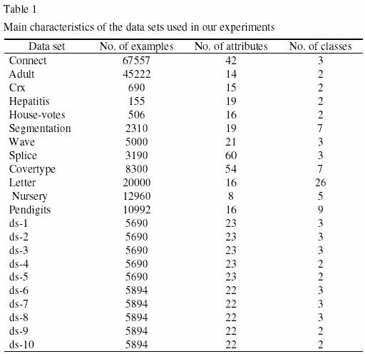
We have extensively evaluated the predictive accuracy of both GA-Small and GA-Large-SN across 22 real-world data sets. 12 of these 22 data sets are publicdomain data sets of the well-known UCI’ s data repository, available at: http://www.ics.uci.edu/~mlearn/MLRepository.html. The other 10 data sets are derived from a database of the CNPq (the Brazilian government’ s National Council of Scientific and Technological Development), whose details are confidential. Some general information about this proprietary database and the corresponding data sets extracted from them is as follows. The database contains data about the scientific production of researchers. We have obtained a subset of this database containing data about a subset of researchers whose data the user was interested in analyzing. This data subset was anonymized before the data mining algorithm was applied – i.e., all attributes that identified a single researcher were removed for data mining purposes. We have identified five possible class attributes in this database – i.e., five attributes whose value the user would like to predict, based on the values of the predictor attributes for a given record (researcher). These class attributes involve information about the number of publications of researchers, with each class attribute referring to a specific kind of publication. For each class attribute, we have extracted two data sets from the database, with a somewhat different set of predictor attributes in the two data sets. This has led to the extraction of 10 data sets, denoted ds-1, ds-2, ds-3, ..., ds-10. The number of examples, attributes and classes for each of the 22 data sets is shown in Table 1.
The examples that had some missing value were removed from these data sets. All accuracy rates reported here refer to results in the test set. In three of the public domain data sets, Adult, Connect and Letter, we have used a single division of the data set into a training and a test set. This is justified by the fact that the data sets are relatively large, so that a single relatively large test set is enough for a reliable estimate of predictive accuracy. In the Adult data set we used the predefined division of the data set into a training and test sets. In the Letter and the Connect data sets, since no such predefined division was available, we have randomly partitioned the data into a training and a test sets. In the Letter the data set, the training and test set had 14000 examples and 6000 examples, respectively. In the Connect data set the training and test sets had 47290 and 20267 examples, respectively. In the other public domain datasets, as well as in the 10 data sets derived from the CNPq’ s database, we have run a well-known 10-fold cross-validation procedure. In essence, the data set is randomly divided into 10 partitions, each of them having approximately the same size. Then the classification algorithm is run 10 times. In the i-th run, i = 1,...,10, the i-th partition is used as the test set and the other 9 partitions are temporarily merged and used as the training set. The result of this cross-validation procedure is the average accuracy rate in the test set over the 10 iterations.
The experiments used C4.5 [24] as the decision-tree component of our hybrid method. We have evaluated two versions of our hybrid method, namely C4.5/GA-Small and C4.5/GA-Large-SN. These versions are compared with two versions of C4.5 alone. The first version simply consists of running C4.5 (with its default parameters) and use the constructed decision tree to classify all examples – i.e., both large-disjunct examples and small-disjunct examples.
The second version consists of a “ double run” of C4.5, hereafter called “ double C4.5“ for short. The latter is a new way of using C4.5 to cope with small disjuncts, whose basic idea is to build a classifier by running C4.5 twice. The first run considers all examples in the original training set, producing a first decision-tree. Once all the examples belonging to small disjuncts have been identified by this decision tree, the system groups all those examples into a single example subset, creating the “ second training set” , as described above for GALarge- SN (see Fig 4(b)). Then C4.5 is run again on this second training set, producing a second decision tree. In other words, the second run of C4.5 uses as training set exactly the same “ second training set” used by GA-Large-SN. In order to classify a new example, the rules discovered by both runs of C4.5 are used as follows. First, the system checks whether the new example belongs to a large disjunct of the first decision tree. If so, the class predicted by the corresponding leaf node is assigned to the new example. Otherwise (i.e., the new example belongs to one of the small disjuncts of the first decision tree), the example is classified by the second decision tree. The motivation for this more elaborated use of C4.5 was an attempt to create a simple algorithm that was more effective in coping with small disjuncts.
In our experiments we have used a commonplace definition of small disjunct, based on a fixed threshold of the number of examples covered by the disjunct. More precisely, a decision-tree leaf is considered a small disjunct if and only if the number of examples belonging to that leaf is smaller than or equal to a fixed size S. We have done experiments with two different values of S, namely S = 10 and S = 15.
We use the term “ experiment” to refer to all the runs performed for all algorithms and for all the above-mentioned 22 data sets, for each value of S (10 and 15). More precisely, each of the two experiments consists of running default C4.5, double C4.5, C4.5/GA-Small and C4.5/GA-Large-SN for the 22 data sets, using a single training/test set partition in the Adult, Connect and Letter data sets and using 10-fold cross-validation in the other 19 data sets. Whenever a GA (GA-Small or GA-Large-SN) was run, that GA was run ten times, varying the random seed used to generate the initial population of individuals. (Obviously, the C4.5 component of the method does not need to be run with different random seeds, only the GA does.) The GA-related results reported below are based on an arithmetic average of the results over these ten different random seeds (in the same way that the cross-validation results are an average of the results over the 10 folds, of course). Therefore, GA-Large-SN’ s and GA-Small’ s results are based on average results over 100 runs (10 seeds x 10 cross-validation folds), except in the Adult, Connect and Letter data sets, where the results were averaged over 10 runs (10 seeds).
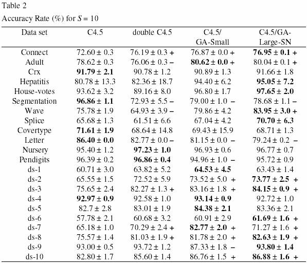
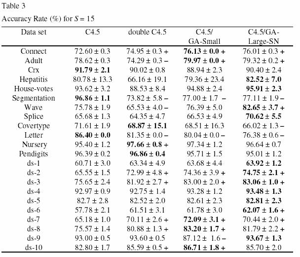
In the two experiments, GA-Small and GA-Large-SN were always run with a population of 200 individuals, and the GA was run for 50 generations. The results of the experiments for S = 10 and S = 15 are reported in Tables 2 and 3, respectively. In these tables the first column indicates the data set, and the other columns report the corresponding accuracy rate in the test set (in %) obtained by default C4.5, double C4.5, C4.5/GA-Small and C4.5/GA-Large-SN. The numbers after the “ r“ symbol denote standard deviations. For each data set, the highest accuracy rate among all the four algorithms is shown in bold. In the third, fourth and fifth columns we indicate, for each data set, whether or not the accuracy rate of double C4.5, C4.5/GA-Small and C4.5/GA-Large-SN, respectively, is significantly different from the accuracy rates of default C4.5. This allows us to evaluate the extent to which those three methods can be considered good solutions for the problem of small disjuncts. More precisely, the cases where the accuracy rate of each of those three methods is significantly better (worse) than the accuracy rate of default C4.5 is indicated by the “ +” (“ -“ ) symbol. A difference between two methods is deemed significant when the corresponding accuracy rate intervals (taking into account the standard deviations) do not overlap. Note that the accuracy rates of default C4.5 in Tables 2 and 3 (where S = 10 and S = 15, respectively) are exactly the same, since C4.5’ s accuracy rates do not depend on the value of S.
Let us first analyze the results of Table 2, where S = 10. Double C4.5 was not very successful. It performed significantly better than default C4.5 in four data sets, but it performed significantly worse than default C4.5 in four data sets as well. A better result was obtained by C4.5/GA-Small. This method was significantly better than default C4.5 in 7 data sets, and it was significantly worse than default C4.5 in 4 data sets. An even better result was obtained by C4.5/GALarge- SN. This method was significantly better than default C4.5 in 9 data sets, and it was significantly worse than default C4.5 in only 2 data sets. In addition, C4.5/GA-Large-SN obtained the best accuracy rate among all the four methods in 11 of the 22 data sets, whereas C4.5/GA-Small was the winner in only 5 data sets.
Let us now analyze the results of Table 3 (where S = 15). Double C4.5 performed significantly better than default C4.5 in 7 data sets, and it performed significantly worse than default C4.5 in four data sets. Somewhat better results were obtained by C4.5/GA-Small and C4.5/GA-Large-SN. C4.5/GA-Small also was significantly better than default C4.5 in 7 data sets, but it was significantly worse than default C4.5 in only 3 data sets. C4.5/GA-Large-SN was significantly better than default C4.5 in 8 data sets, and it was significantly worse than default C4.5 in only 3 data sets. Again, C4.5/GA-Large-SN obtained the best accuracy rate among all the four methods in 11 of the 22 data sets, whereas C4.5/GA- Small was the winner in only 5 data sets.
Finally, a comment on computational time is appropriate here. We have mentioned, in section 3.2, that one of our motivations for designing GA-Large- SN was to reduce processing time, by comparison with GA-Small. In order to validate this point, we have done an experiment comparing the processing time of C4.5/GA-Large-SN and GA-Small on the same machine (a Pentium III with 192 MB of RAM) in the largest data set used in our experiments, the Connect data set. In this data set C4.5/GA-Small ran in 50 minutes, whereas C4.5/GALarge- SN ran in only 6 minutes, confirming that GA-Large-SN tends to be considerably faster than GA-Small. In the same data set and on the same machine C4.5 alone ran in 44 seconds, and double C4.5 ran in 52 seconds. Although C4.5/GA-Large-SN is still slower than C4.5 alone and double C4.5, we believe the increase in computational time associated with C4.5/GA-Large-SN is not too excessive, and it is a small price to pay for its associated increase in predictive accuracy. In addition, it should be noted that predictive data mining is typically an off-line task, and it is well-known that in general the time spent with running a data mining algorithm is a small fraction (less than 20%) of the total time spent with the entire knowledge discovery process. Data preparation is usually the most time consuming phase of this process. Hence, in many applications, even if a data mining algorithm is run for several hours or several days, this can be considered an acceptable processing time, at least in the sense that it is not the bottleneck of the knowledge discovery process.
Liu et al. present a new technique for organizing discovered rules in different levels of detail [18]. The algorithm consists of two steps. The first one is to find top-level general rules, descending down the decision tree from the root node to find the nearest nodes whose majority classes can form significant rules. They call these rules the top-level general rules. The second is to find exceptions, exceptions of the exceptions and so on. They determine whether a tree node should form an exception rule or not using two criteria: significance and simplicity. Some of the exception rules found by this method could be considered as small disjuncts. However, unlike most of the projects discussed below, the authors do not try to discover small-disjuncts rules with greater predictive accuracy. Their method was proposed only as a form of summarizing a large set of discovered rules. By contrast our work aims at discovering new small-disjunct rules with greater predictive power than the corresponding rules discovered by a decision tree algorithm. Next we discuss other projects more related to our research.
Weiss and Hirsh present a quantitative measure for evaluating the effect of small disjuncts on learning [30]. The authors reported experiments with a number of data sets to assess the impact of small disjuncts on learning, especially, when factors such as training set size, pruning strategy, and noise level are varied. Their results confirmed that small disjuncts do have a negative impact on predictive accuracy in many cases. However, they did not propose any solution for the problem of small disjuncts.
Holte et al. investigated three possible solutions for eliminating small disjuncts without unduly affecting the discovery of “ large” (non-small) disjuncts [17], namely: (a) Eliminating all rules whose number of covered training examples is below a predefined threshold. In effect, this corresponds to eliminating all small disjuncts, regardless of their estimated performance. (b) Eliminating only the small disjuncts whose estimated performance is poor. Performance is estimated by using a statistical significance test. (c) Using a specificity bias for small disjuncts (without altering the bias for large disjuncts). Ting proposed the use of a hybrid data mining method to cope with small disjuncts [27]. His method consists of using a decision-tree algorithm to cope with large disjuncts and an instance-based learning (IBL) algorithm to cope with small disjuncts. The basic idea of this hybrid method is that IBL algorithms have a specificity bias, which should be more suitable for coping with small disjuncts. Similarly, Lopes and Jorge discuss two techniques for rule and case integration [19]. Case-based learning is used when the rule base is exhausted. Initially, all the examples are used to induce a set of rules with satisfactory quality. The examples that are not covered by these rules are then handled by a case-based learning method. In this proposed approach, the paradigm is shifted from rule learning to case-based learning when the quality of the rules gets below a given threshold. If the initial examples can be covered with high-quality rules the casebased approach is not triggered. In a high level of abstraction, the basic idea of these two methods is similar to our hybrid decision-tree/genetic algorithm method. However, these two methods have the disadvantage that the IBL (or CBL) algorithm does not discover any high-level, comprehensible rules. By contrast, we use a genetic algorithm that does discover high-level, comprehensible small-disjunct rules, which is important in the context of data mining.
Weiss investigated the interaction of noise with rare cases (true exceptions) and showed that this interaction led to degradation in classification accuracy when small-disjunct rules are eliminated [28]. However, these results have a limited utility in practice, since the analysis of this interaction was made possible by using artificially generated data sets. In real-world data sets the correct concept to be discovered is not known a priori, so that it is not possible to make a clear distinction between noise and true rare cases. Weiss did experiments showing that, when noise is added to real-world data sets, small disjuncts contribute disproportional and significantly for the total number of classification errors made by the discovered rules [29].
In this paper we have described two versions of a hybrid decision tree (C4.5)/genetic algorithm (GA) solution for the problem of small disjuncts. The two versions involve two different GAs, namely GA-Small and GA-Large-SN. We have compared the performance of the two versions of our method, C4.5/GA-Small and C4.5/GA-Large-SN, with the performance of two methods based on C4.5 alone, namely C4.5 and "double C4.5".
Overall, taking into account the predictive accuracy in 22 data sets (see Tables 2 and 3), the best results were obtained by the hybrid method C4.5/GA-Large- SN. Hence, this method can be considered as a good solution for the smalldisjunct problem – which, as explained in the Introduction, is a challenging problem in classification research.
In this paper we have compared our hybrid decision tree/GA methods with C4.5 alone. In future research we intend to compare these hybrid methods with a GA alone as well. We also intend to compare our hybrid decision tree/GA methods with other kinds of hybrid methods, such as the hybrid decision tree / instance-based learning method proposed by [27].
[1] D. Beasley, D. R. Bull, R. R. A. Martin, Sequential Niche Technique for Multimodal Function Optimization. Evolutionary Computation 1(2), 1993, 101-125. MIT Press.
[2] T. Blickle, Tournament selection. In: T. Back, D.B. Fogel and T. Michalewicz. (Eds.) Evolutionary Computation 1: Basic Algorithms and Operators, 2000, 181-186. Institute of Physics Publishing.
[3] D. R. Carvalho, A. A. Freitas, A hybrid decision tree/genetic algorithm for coping with the problem of small disjuncts in Data Mining. Proc 2000 Genetic and Evolutionary Computation Conf. (Gecco-2000), 2000, 1061-1068. Las Vegas, NV, USA. July.
[4] D. R. Carvalho, A. A. Freitas, A genetic algorithm-based solution for the problem of small disjuncts. Principles of Data Mining and Knowledge Discovery (Proc. 4th European Conf., PKDD-2000. Lyon, France). Lecture Notes in Artificial Intelligence 1910, 2000, 345-352. Springer-Verlag.
[5] D.R. Carvalho and A.A. Freitas. A genetic algorithm with sequential niching for discovering smalldisjunct rules. Proc. Genetic and Evolutionary Computation Conf. (GECCO-2002), pp. 1035-1042. Morgan Kaufmann, 2002.
[6] D.R. Carvalho and A.A. Freitas. A genetic algorithm for discovering small-disjunct rules in data mining. Applied Soft Computing, in press. 2002.
[7] Cohen, W.W., Efficient pruning methods for separate-and-conquer rule learning systems. Proc. 13th Int. Joint Conf. on Artif. Intel. (IJCAI-93), 1993, 988-994.
[8] T. M. Cover, J. A. Thomas, Elements of Information Theory. John Wiley&Sons, 1991.
[9] V. Dhar, D. Chou, F. Provost, Discovering Interesting Patterns for Investment Decision Making with GLOWER – A Genetic Learner Overlaid With Entropy Reduction. Data Mining and Knowledge Discovery 4(4), Oct. 2000., 251-280.
[10] A. P. Danyluk, F. J. Provost, Small Disjuncts in Action: Learning to Diagnose Erros in the Local Loop of the Telephone Network, Proc. 10th International Conference Machine Learning, 1993, 81-88.
[11] A. A. Freitas, Understanding the crucial role of attribute interaction in data mining. Artificial Intelligence Review 16(3), Nov. 2001, 2001, 177-199.
[12] A. A. Freitas, Evolutionary Algorithms. Chapter of forthcoming Handbook of Data Mining and Knowledge Discovery. Oxford University Press, 2002.
[13] A.A. Freitas. Data Mining and Knowledge Discovery with Evolutionary Algorithms. Berlin: Springer-Verlag, 2002.
[14] D. E. Goldberg, J. Richardson, Genetic Algorithms with Sharing for Multimodal Function Optimization. Proc. Int. Conf. on Genetic Algorithms (ICGA-87), 1987, 41-49.
[15] D. P. Greene, S. F. Smith, Competition-based induction of decision models from examples. Machine Learning, 13, 1993. 229-257.
[16] D. J. Hand, Construction and Assessment of Classification Rules, John Wiley & Sons, 1997.
[17] R. C. Holte, L. E. Acker, B. W. Porter, Concept Learning and the Problem of Small Disjuncts, Proc. IJCAI – 89, 1989, 813-818.
[18] B. Liu, M. Hu, W. Hsu, Multi-level Organization and Summarization of the Discovered Rules, Proc. 6th ACM SIGKDD Int. Conf. On Knowledge Discovered & Data Mining (KDD– 2000), 2000. 208-217.
[19] A. A. Lopes, A. Jorge, Integrating Rules and Cases in Learning via Case Explanation and Paradigm Shift, Advances in Artificial Intelligence. (Proc. IBERAMIA – SBIA 2000). LNAI 1952, 33-42. 2000.
[20] S. W. Mahfoud, Niching Methods for Genetic Algorithms, Illigal Report N. 95001, Thesis Submitted for degree of Doctor of Philosophy in Computer Science. University of Illinois at Urbana-Champaign, 1995
[21] Z. Michalewicz, Genetic Algorithms + Data Structures = Evolution Programs. 3rd Ed. Springer- Verlag, 1996.
[22] A. Papagelis, D. Kalles, Breeding decision trees using evolutionary techniques. Proc. 18th Int. Conf. on Machine Learning (ICML-2001), 393-400. Morgan Kaufmann, 2001.
[23] J.R. Quinlan, Learning logical definitions from relations. Machine Learning 5(3), 1990. 239-266.
[24] J. R. Quinlan, C4.5: Programs for Machine Learning, Morgan Kaufmann Publisher, 1993.
[25] L. Rendell, R. Seshu, Learning hard concepts through constructive induction: framework and rationale. Computational Intelligence 6, 1990, 247-270.
[26] L. Rendell, H. Ragavan, Improving the design of induction methods by analyzing algorithm functionality and data-based concept complexity. Proc. 13th Int. Joint Conf. on Artif. Intel. (IJCAI-93), 1993. 952-958.
[27] K. M. Ting, The Problem of Small Disjuncts: its remedy in Decision Trees, Proc. 10th Canadian Conference on AI, 1994. 91-97.
[28] G. M. Weiss, Learning with Rare Cases and Small Disjuncts, Proc. 12th International Conference on Machine Learning (ICML-95), 1995. 558-565.
[29] G. M. Weiss,, The Problem with Noise and Small Disjuncts, Proc. Int. Conf. Machine Learning (ICML – 98), 1998, 574-578.
[30] G. M. Weiss, H. Hirsh, A Quantitative Study of Small Disjuncts, Proc. of Seventeenth National Conference on Artificial Intelligence (AAAI-2000). Austin, Texas, 2000. 665-670.