Source: http://www.cmis.csiro.au/Hugues.Talbot/dicta2003/cdrom/pdf/0089.pdf
Hanzi Wang and David Suter
Department of. Electrical. and Computer Systems Engineering Monash University, Clayton
3800, Victoria, Australia
mailto:hanzi@eng.monash.edu.au
mailto:wang@eng.monash.edu.au
Abstract. This paper proposes a new method of color image segmentation considering both global information and local homogeneity. The method applies the mean shift algorithm in the hue and intensity subspace of HSV. The cyclic property of the hue component is also considered in the proposed method. Experiments on natural color images show promising results.
One major task of pattern recognition, image processing, and related areas: is to segment image into homogenous regions. Image segmentation is the first step towards image understanding and image analysis. Image segmentation has been acknowledged to be one of the most difficult tasks in computer vision and image processing [3, 8]. Unlike other vision tasks such as parametric model estimation [20, 22], fundamental matrix estimation [18], optical flow calculation [21], etc., there is no widely accepted model or analytical solution for image segmentation. There probably is no “one true” segmentation acceptable to all different people and under different psychophysical conditions.
A lot of image segmentation methods have been proposed: roughly speaking, these methods can be classified into [3]: (1) Histogram thresholding [13]; (2) Clustering [6, 23, 2]; (3) Region growing [1]; (4) Edge-based [14]; (5) Physicalmodel- based [12]; (6) Fuzzy approaches [15]; and (7) Neural network methods [11].
Clustering techniques identify homogeneous clusters of points in the feature space (such as RGB color space, HSV color space, etc.) and then label each cluster as a different region. The homogeneity criterion is usually that of color similarity, i.e., the distance from one cluster to another cluster in the color feature space should be smaller than a threshold. The disadvantage of this method is that it does not consider local information between neighboring pixels.
In this paper, we propose a segmentation method introducing local homogeneity into a mean shift algorithm: using both global and local information. The method is performed in "Hue-Value" two-dimensional subspace of Hue-Saturation-Value space. Compared with applying the mean shift algorithm in LUV or RGB color space, the complexity of the proposed method is lower. The proposed method also considers the cyclic property of the hue component, does not need priori knowledge about the number of cluster, and it detects the clusters unsupervised.
The paper is organized as follows: in section 2, HSV color space is introduced; the mean shift algorithm is introduced in section 3. The proposed color image segmentation method is given in section 4. Section 5 includes experiments on color image (real) segmentation. The conclusion can be found in section 6.
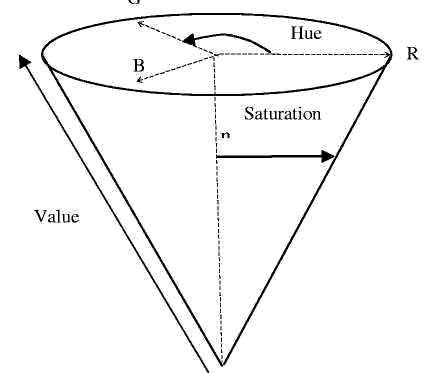
RGB (Red, Green, and Blue) is a widely used color space but HSV (Hue, Saturation, and Value) is sometimes preferred (see Figure 1). Hue, is a specification of the intrinsic color. Saturation, describes, “how pure the color is”. The last component of the HSV triple is a measure of “how bright the color is”. The HSI (hue-saturationintensity), the HSB (hue-saturation-brightness), and the HSL (hue-saturationlightness) are variant forms of the HSV color space [3]. HSV has been widely used in computer vision tasks [4, 23, 17]. The advantages of HSV over RGB are [4, 3]:
Although the authors of [4] utilized both hue and intensity to segment color images, they segmented color images in one-dimensional intensity subspace and then, hierarchically, segmented the results (from the segmentation in the intensity subspace) in the hue subspace. Thus it is easy to over-segment the image. In this paper, we apply the mean shift algorithm in hue-value two-dimensional subspace. The hue and value are scaled ranging from 0 to 255. Because the hue is a value of angle, it has a cyclic property (see subsection 3.3 and 4.2).
Figure 1. HSV color space.
Since Fukunaga and Hostetler [10] introduced the mean shift algorithm, the mean shift algorithm has been extensively exploited and applied in low-level computer vision tasks [5, 7, 8] for its ease and efficiency. One characteristic of the mean shift vector is that it always points towards the direction of the maximum increase in the density. The converged centers (or windows) correspond to modes (or centers of the regions of high concentration) of data. The mean shift algorithm is based on kernel density estimation.
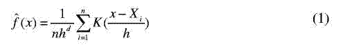
Let {Xi}i=1,...,n be a set of n data points in a d-dimensional Euclidian space Rd, the multivariate kernel density estimator with kernel K and window radius (band-width) h is defined as follows ([16], p.76):
The kernel function K(x) should satisfy some conditions ([19], p.95). The Epanechnikov kernel ([16], p.76) is one optimum kernel, which yields minimum mean integrated square error (MISE):
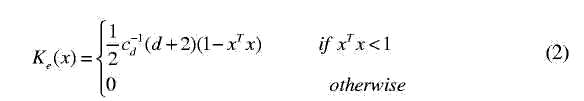
where cd is the volume of the unit d-dimensional sphere, e.g., c1=2, c2= , c3=4 /3. Thus, the density gradient estimate of the Epanechnikov kernel can be written as:
Equation (3) can be rewritten as:
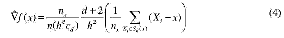
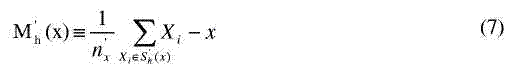
where the region Sh(x) is a hypersphere of the radius h, having the volume , centered at x, and containing nx data points. The mean shift vector Mh(x) is defined as:
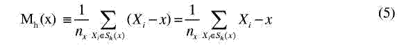
From equation (4) and equation (5), we get:
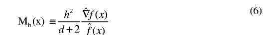
Equation (6) firstly appeared in [10]. The mean shift is an unsupervised nonparametric estimator of density gradient and the mean shift vector is the difference between the local mean and the center of the window.
The Mean Shift algorithm can be described as follows:
The mean shift automatically finds the local maximum density. This property holds even in high dimensional feature spaces. In [4], the authors also proposed a peak-finding algorithm. Unfortunately, it is heuristically based. In contrast, the mean shift algorithm has a solid theoretical foundation. The proof of the convergence of the mean shift algorithm can be found in [7, 8].
Because the hue is a value of angle, the cyclic property of the hue must be considered. The revised mean shift algorithm can be written as:
where the converging window center x is a vector of [H, V],
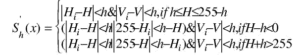
and nx is the number of data points inside the hypersphere Sh(x).
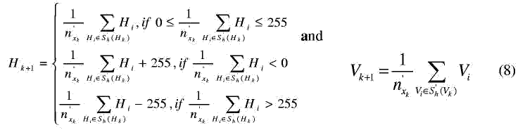
When translating the search window, let xk+1=[Hk+1,Vk+1]. We have:
Although the mean shift algorithm has been successfully applied to clustering [5, 7], image segmentation [6, 8], tracking [9], etc., it considers only global information, while neglecting local information. In this paper, we introduce a measure of local homogeneity [4] into the mean shift algorithm. The proposed method considers both global information and local homogeneity information.
In [4], a measure of local homogeneity has been used in one-dimensional histogram thresholding. The homogeneity consists of two parts: the standard deviation and the discontinuity of the intensities at each pixel of the image. The standard derivation Sij at pixel Pij can be written as:
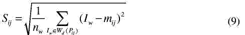
where mij is the mean of nw intensities within the window Wd(Pij), which has a size of d by d and is centered at Pij.
A measure of the discontinuity Dij at pixel Pij can be written as:
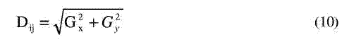
where Gx and Gy are the gradients at pixel Pij in the x and y direction.
Thus, the homogeneity Hij at Pij can be written as:

From equation (11), we can see that the H value ranges from 0 to 1. The higher the Hij value is, the more homogenous the region surrounding the pixel Pij is.
In [4], the authors applied this measure of homogeneity to the histogram of gray levels. In this paper, we will show that the local homogeneity can also be incorporated into the popular mean shift algorithm.
Our proposed method mainly consists of three parts:
The details of the proposed method are:
1. Map the image to the feature space. We first compute the local homogeneity value at each pixel of the image. To calculate the standard variance at each pixel, a 5-by-5 window is used. For the discontinuity estimation, we use a 3-by-3 window. Of course, other window sizes can also be used. However, we find that the window sizes used in our case can achieve better performance and computational efficiency.
After computing the homogeneity for each pixel, we only use the pixels with high homogeneity values (near to 1.0) and neglect the pixels with low homogeneity values. We map the pixels with high homogeneity values into the hue-value two-dimensional space. Thus, both global and local information are considered.
2. Apply the mean shift algorithm to find the local high-density modes. We randomly initialize some windows in HV space, with radius h. When the number of data points inside the window is large, and when the window center is not too close to the other accepted windows, we accept the window. After the initial window has been chosen, we apply the mean shift algorithm considering the cyclic property of the hue component to obtain the local peaks.
3. Validate the peaks and label the pixels. After applying the mean shift algorithm, we obtain a lot of peaks. Obviously, these peaks are not all valid. We need some postprocessing to validate the peaks.
1) Eliminate the repeated peaks. Because of the limited accuracy of the mean shift, the same peak obtained by the mean shift may not be at the exact same location. Thus, we remove the repeated peaks that are very close to each other (e.g., their distance is less than 1.0).
2) Remove the small peaks related to the maximum peaks. Because the mean shift algorithm only finds the local peaks, it may stop at small local peaks. Calculate the normalized contrast for two neighboring peaks and the valley between the two peaks:
where the contrast is the difference between the smaller peak and the valley; the height is that of the smaller peaks. Remove the smaller one of the two peaks if this ratio is small.
This step can remove the peaks obtained by the mean shift, which may be at the local plateau of the probability density.
After obtaining the validated peaks, we assign pixels to its nearest clusters. In this step, the cyclic property of the hue component will again be considered. The distance between the i’th pixel to the j’th cluster is:

where a is a factor to adjust the relative weight of the hue component over the value component.
The authors of [23] employed the k-means algorithm to segment image. The disadvantage of such an approach is the requirement that the user must specify the number of the clusters. In comparison, the proposed method is unsupervised and needs no priori knowledge about the number of the clusters.
In the next section, we will show the achievement of the proposed method.
We test our color image segmentation method on natural color images. In Figure 2, part of the procedures of the proposed method is illustrated and final segmentation results are given. Figure 2 (a) includes the original image “home”. The points in HV space are displayed in Figure 2 (b) (no validation of local homogeneity) and (c) (after validation of local homogeneity). The tracks the mean shift algorithm in HV space, with different initializations, are included in Figure 2 (d). The blue lines are the traces of the mean shift procedures; green dots are the centers of the converged windows by the mean shift procedures; and the red circles are the final peaks after validation. Figure 2 (e) gives the final segmentation results by the proposed method. From Figure 2 (e), we can see that our method obtains good segmentation results. The tree, the house, the roof, and the rim of curtain and house are all segmented out separately. The curtain and the sky are segmented to the same cluster. This is because the color of the curtain is blue, which is similar to the color of sky. From the point of view for color homogeneity, this result is correct.
We also note that the grassland are segmented into two parts: on one hand, one can say the method over-segments the grassland because they both belong to the grassland; on the other hand, one can say the method correctly segment the grassland because the grassland can be seen to have different colors. This again demonstrates that there is no unique solution to image segmentation.
In and Figure 4, we compare the proposed method with a method employing a similar scheme but without considering the local homogeneity and the cyclic property of the hue component.
From , we can see that the method without considering the local homogeneity and the cyclic property of the hue component over-segments the image of “Jelly beans” into seven colors; the blue beans fall into two clusters; part of the red beans are wrongly assigned to the black beans. In contrast, the proposed method correctly segments the “Jelly beans” images into five colors (four colors from beans and one color from background).
In Figure 4, we can see that the method without considering the local homogeneity and the cyclic property of the hue component over-segments the image of “Splash”. The red background falls into two clusters; also, some pixels of the red background are wrongly assigned to the object in the image. In contrast, the proposed method considering the local homogeneity and the cyclic property of the hue component obtains good results. The image is effectively compressed to three colors.
In this paper, we propose a novel color image segmentation method. We employ the concept of homogeneity, and the mean shift algorithm, in our method. Thus the proposed method considers both local and global information in segmenting the image into homogenous regions. We segment the image in the hue-value twodimensional feature space. Thus, the computational complexity is reduced, compared with the methods that segment image in LUV or RGB three-dimensional feature space. The cyclic property of the hue component is considered in the mean shift procedures and in the labeling of the pixels of the image. Experiments show that the proposed method achieves promising results for natural color image segmentation.
1. Adams, R. and L. Bischof, Seeded Region Growing. IEEE Trans. Pattern Analysis and Machine Intelligence, 1994. 16: p. 641-647. 2. Chen, T.Q. and Y. Lu, Color Image Segmentation--An Innovative Approach. Pattern Recognition, 2001. 35: p. 395-405.
3. Cheng, H.D., et al., Color Image Segmentation: Advances and Prospects. Pattern Recognition, 2001. 34: p. 2259-2281.
4. Cheng, H.D. and Y.Sun, A Hierarchical Approach to Color Image Segmentation Using Homogeneity. IEEE Trans. Image Processing, 2000. 9(12): p. 2071-2082.
5. Cheng, Y., Mean Shift, Mode Seeking, and Clustering. IEEE Trans. Pattern Analysis and Machine Intelligence, 1995. 17(8): p. 790-799.
6. Comaniciu, D. and P. Meer, Robust Analysis of Feature Spaces: Color Image Segmentation. in Proceedings of 1997 IEEE Conference on Computer Vision and Pattern Recognition, San Juan, PR, 1997: p. 750-755.
7. Comaniciu, D. and P. Meer, Distribution Free Decomposition of Multivariate Data. Pattern Analysis and Applications, 1999. 2: p. 22-30.
8. Comaniciu, D. and P. Meer, Mean Shift: A Robust Approach towards Feature Space A Analysis. IEEE Trans. Pattern Analysis and Machine Intelligence, 2002. 24(5): p. 603-619.
9. Comaniciu, D., V. Ramesh, and P. Meer. Real-Time Tracking of Non-Rigid Objects using Mean Shift. in IEEE Conf. Computer Vision and Pattern Recognition. 2000: p. 142-149.
10.Fukunaga, K. and L.D. Hostetler, The Estimation of the Gradient of a Density Function, with Applications in Pattern Recognition. IEEE Trans. Info. Theory, 1975. IT-21: p. 32-40.
11.Iwata, H. and H. Nagahashi, Active Region Segmentation of Color Image Using Neural Networks. Systems Comput. J., 1998. 29(4): p. 1-10.
12.Klinker, G.J., S.A. Shafer, and T. Kanade, A Physical Approach to Color Image Understanding. International Journal of Computer Vision, 1990. 4: p. 7-38.
13.Kurugollu, F., B. Sankur, and A.E. Harmani, Color Image Segmentation Using Histogram Multithresholding and Fusion. Image and Vision Computing, 2001. 19: p. 915-928.
14.Nevatia, A Color Edge Detector and Its Use in Scene Segmentation. IEEE TRans. System Man Cybernet, 1977. SMC-7(11): p. 820-826.
15.Pal, S.K., Image Segmentation Using Fuzzy Correlation. Inform. Sci., 1992. 62: p. 223-250.
16.Silverman, B.W., Density Estimation for Statistics and Data Analysis. 1986, London: Chapman and Hall.
17.Sural, S., G. Qian, and S. Pramanik. Segmentation and Histogram Generation Using the HSV Color Space for Image Retrieval. in International Conference on Image Processing (ICIP). 2002: p. 589-592.
18.Torr, P. and D. Murray, The Development and Comparison of Robust Methods for Estimating the Fundamental Matrix. International Journal of Computer Vision, 1997. 24: p. 271-300.
19.Wand, M.P. and M. Jones, Kernel Smoothing. Chapman & Hall, 1995.
20.Wang, H. and D. Suter. A Novel Robust Method for Large Numbers of Gross Errors. in Seventh International Conference on Control, Automation, Robotics And Vision (ICARCV02). 2002. Singapore: p. 326-331.
21.Wang, H. and D. Suter. Variable bandwidth QMDPE and its application in robust optic flow estimation. in Proceedings ICCV03, International Conference on Computer Vision. 2003. Nice, France: p. to appear.
22.Wang, H. and D. Suter, Using Symmetry in Robust Model Fitting. Pattern Recognition Letters, 24(16): p. 2953-2966, 2003.
23. Zhang, C. and P.Wang. A New Method of Color Image Segmentation Based on Intensity and Hue Clustering. in International Conference on Pattern Recognition (ICPR). 2000: p. 613-616.
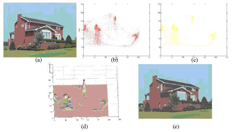
Figure 2. (a) the original image “home”; (b) The hue-value feature space without considering local homogeneity; (c) The hue-value feature space considering local homogeneity; (d) procedures and results of the data decomposition by the mean shift algorithm with different initializations (e) the final results with seven colors obtained by the proposed method with h=9.

Figure 3. (a) the original image “Jelly beans”; (b) the final results with five colors obtained by the proposed method with h=7; (c) the results with seven colors without considering the local homogeneity and the cyclic property of the hue (h=7).

Figure 4. (a) the original image “Splash”; (b) the final results with three colors obtained by the proposed method with h=7; (c) the results with six colors without considering the local homogeneity and the cyclic property of the hue (h=7).