DISJUNCTIVE SCHEDULING

Jobshop scheduling

      A scheduling problem is defined by a set of tasks T and a set of resources R. Tasks are constrained by precedence relationships, which bind some tasks to wait for other ones to complete before they can start. Tasks that share a resource are not interruptible (non-preemptive scheduling) and mutually exclusive (disjunctive versus cumulative scheduling). The goal is to find a schedule that performs all tasks in the minimum amount of time.
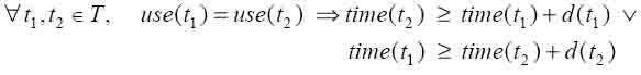
      Formally, to each task t , a non-negative duration d(t) and a resource use(t) are associated. For precedence relations, precede(t1, t2 ) denotes that t₂ cannot be performed before t₁ is completed. The problem is then to find a set of starting times {time(t)}, that minimizes the total makespan of the schedule defined as Makespan := max{time(t) + d(t)} under the following constraints:



       Job-shop scheduling is a special case where the tasks are grouped into jobs j¹,..., jⁿ . A job jⁱ is a sequence of tasks j₁ⁱ,..., j_mⁱ that must be performed in this order, i.e., for all , one has precede( j_kⁱ , j_k+1ⁱ). Such problems are called n x m problems, where n is the number of jobs and m the number of resources. The precedence network is thus very simple: it consists of n “chains”. The simplification does not come from the matrix structure (one could always add empty tasks to a scheduling problem) but rather from the fact that precedence is a functional relation. It is also assumed that each task in a job needs a different machine. For a task j_kⁱ , the head will be defined as the sum of the durations of all its predecessors on its job and similarly the tail as the sum of the durations of all its successors on its job, e.g.:


       When one allows the precedence relations to form a more complex network, the problem is referred to as a disjunctive scheduling problem. Although general disjunctive scheduling problems are often more appropriate for modelling real-life situations, little work concerning them has been done (they have been studied more by the AI community than by Operations Researchers and most of the published work concerns small instances, like a famous bridge construction problem with 42 tasks [VH89]) The interest of n x m scheduling problems is the attention they have received in the last 30 years. The most famous instance is a 10 x 10 problem of Fisher & Thompson [MT63] that was left unsolved until 1989 when it was solved by Carlier & Pinson [CP89]. Classical benchmarks include problems randomly generated by Adams, Balas & Zawak in 1988 [ABZ88], Applegate & Cook in 1990 [AC91] and by Lawrence in 1984 [La84]. Of the 40 problems published by Lawrence, one is still unsolved (a 20 x 10 referred to as LA29). The typical size of these benchmarks ranges from 10 x 5 to 30 x 10.

The branch and bound scheme with time windows

      Branch and bound algorithms have, however, undergone much study, and the method effectively used in [CP89] to solve MT10 is a branch & bound scheme called “edge-finding”. Since a schedule is a set of orderings of tasks on the machines, a natural way to compute them step after step is to order a pair of tasks that share the same resource at each node of the search tree (which corresponds to getting rid of a disjunction in the constraint formulation). There are many variations depending on which pair to pick, how to exploit the disjunctive constraint before the pair is actually ordered, etc., but the general strategy is almost always to order pairs of tasks [AC91].
      The domain associated with time(t_i) is represented as an interval : to each task t_i, a window [t_i, ¯t_i - d(t_i)] is associated, where t_i is the minimal starting date and t_i is the maximal completion date (thus the starting date time(t_i) must be between t_i and t_i-d(t_i )). During the search, a partial ordering (<<) of tasks is built, with the following meaning : t₁ << t₂<=>time(t₁)+d(t₁)<=time(t₂)
      In order to prune efficiently the search space, one needs to be able to propagate the decisions taken at each node of the search tree. Thus, whenever an ordering is selected, say t₁ << t₂, the bounds of the domains can be updated as follows: t₂ >= t₁ + d(t₁) and t₁ <= t₂ - d(t₂). With this model, inconsistency can be detected when one has ¯t - t < d(t) for some task t (t can no longer fit in its window).