SELECTION OF PARAMETERS FOR TEXTURE ANALYSIS FOR THE CLASSIFICATION OF CAROTID PLAQUES
C.I. Christodoulou 1,2, C.S. Pattichis 1, E. Kyriacou 1,2, A. Nicolaides 2
1Department of Computer Science, University of Cyprus, 75 Kallipoleos Str., P.O.Box 20578, 1678 Nicosia, Cyprus
2 Cyprus Institute of Neurology and Genetics, P.O.Box 3462, 1683 Nicosia, Cyprus
email: {cschr2, pattichi, ekyriac}@ucy.ac.cy
Abstract: Texture features extracted from high-resolution ultrasound images of carotid plaques can be used for the identification of patients at risk of stroke. This work explores the selection of the parameters for the computation of the texture features, which will yield the best class separation between symptomatic and asymptomatic subjects. The following texture algorithms were investigated on 230 carotid plaque images (recorded from 115 symptomatic and 115 asymptomatic subjects): Spatial Gray Level Dependence Matrices (SGLDM), Gray Level Difference Statistics (GLDS), Neighbourhood Gray Tone Difference Matrix (NGTDM), Statistical Feature Matrix (SFM) and Laws Texture Energy Measures (TEM). The results in this work show that an optimized texture parameter selection may improve the diagnostic yield.
Introduction
It has been shown [1] that texture features extracted from high-resolution ultrasound images of atherosclerotic carotid plaques can be used for the identification of individuals with asymptomatic carotid stenosis at risk of stroke. In this work the selection of the algorithmic parameters for texture computation is investigated which will lead to better separation between the following two carotid plaque classes: (i) symptomatic because of ipsilateral hemispheric symptoms, and (ii) asymptomatic because they were not connected with ipsilateral hemispheric events.
Materials and Methods
A total of 230 carotid plaque images (115 symptomatic + 115 asymptomatic) were processed. The plaque segments were outlined manually by the expert physician and were used for texture feature extraction and classification. Figure 1 shows an ultrasound image of the carotid artery bifurcation with the atherosclerotic plaque region outlined.
Texture contains important information, which is used by humans for the interpretation and the analysis of many types of images. Texture refers to the spatial interrelationships and arrangement of the basic elements of an image [2]. In this study, the following six different texture feature sets (a total number of 46 features) were extracted from the manually segmented plaques. The texture features were computed several times by varying their texture parameters.
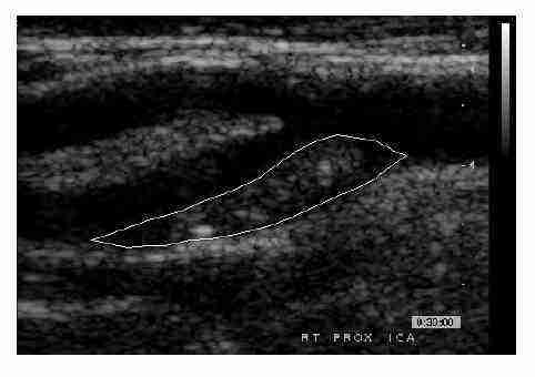
Figure 1: An ultrasound image of the carotid artery bifurcation with the atherosclerotic plaque region outlined.
(i) Spatial Gray Level Dependence Matrices (SGLDM)
The spatial gray level dependence matrices as proposed by Haralick et al. [3] are based on the estimation of the second-order joint conditional probability density functions that two pixels (k,l) and (m,n) with distance d in direction specified by the angle ?, have intensities of gray level i and gray level j. Based on the probability density functions the following texture measures [3] were computed: 1) Angular second moment, 2) Contrast, 3) Correlation, 4) Sum of squares: variance, 5) Inverse difference moment, 6) Sum average, 7) Sum variance, 8) Sum entropy, 9) Entropy, 10) Difference variance, 11) Difference entropy, and 12), 13) Information measures of correlation. For a chosen distance d (e.g. if d=1 then 3x3 matrices) and for angles ? = 0o, 45o, 90o and 135o we computed four values for each of the above 13 texture measures. In this work, the mean and the range of these four values were computed for each feature, and they were used as two different feature sets. The distance parameter d was varied for values 1 to 5.
(ii) Gray Level Difference Statistics (GLDS)
The GLDS algorithm [4] uses first order statistics of local property values based on absolute differences between pairs of gray levels or of average gray levels in order to extract the following texture measures: 1) Homogeneity 2) Contrast, 3) Angular second moment, 4) Entropy, and 5) Mean. The above features were calculated for displacements ? = (0, d), (d, d), (d, 0), (d, -d), where ? ? (?x,?y), and their mean values were taken. The parameter d was varied for values 1 to 5.
(iii) Neighborhood Gray Tone Difference Matrix (NGTDM)
Amadasun and King [2] proposed the Neighborhood Gray Tone Difference Matrix in order to extract textural features, which correspond to visual properties of texture. The following features were extracted, for a neighborhood size of (2d+1)x(2d+1) where d was varied for values 1 to 5: 1) Coarseness, 2) Contrast, 3) Busyness, 4) Complexity, and 5) Strength.
(iv) Statistical Feature Matrix (SFM)
The statistical feature matrix [5] measures the statistical properties of pixel pairs at several distances within an image, which are used for statistical analysis. Based on the SFM the following texture features were computed: 1) Coarseness, 2) Contrast, 3) Periodicity, and 4) Roughness. The constants Lr, Lc which determine the maximum intersample spacing distance were varied for values Lr=Lc=2 to 5, 10 and 15.
(v) Laws Texture Energy Measures (TEM)
For the Laws TEM extraction [6], [7], vectors of lengths l=3, 5 and 7 were examined. For l=3, L=(1, 2, 1), E=(-1, 0, 1), and S=(-1, 2,-1); for l=5, L=(1, 4, 6, 4, 1), E=(-1,-2, 0, 2, 1), S=(-1, 0, 2, 0,-1); and for l=7, L=(1, 6, 15, 20, 15, 6, 1), E=(-1 -4,-5, 0, 5, 4, 1) and S=(-1, -2, 1, 4, 1, -2, -1), where the L vector performs local averaging, E acts as edge detector and S acts as spot detector. If we multiply the column vectors of length l by row vectors of the same length, we obtain Laws lxl masks. In order to extract texture features from an image, these masks are convoluted with the image and the statistics (e.g. energy) of the resulting image are used to describe texture. The following texture features were extracted: 1) LL - texture energy from LL kernel, 2) EE - texture energy from EE kernel, 3) SS - texture energy from SS kernel, 4) LE - average texture energy from LE and EL kernels, 5) ES - average texture energy from ES and SE kernels, and 6) LS - average texture energy from LS and SL kernels.
All features were normalized before use by subtracting their mean value and dividing with their standard deviation.
The extracted features were individually tested for class separability by computing the distance between the two classes for each feature as

where m1 and m2 are the mean values, and ?1 and ?2 are the standard deviations of the two classes. Best features are considered to be the ones with the greatest distance. Although there were individual features that exhibited improved class separability when varying the texture parameters this was not further investigated since it was decided that whole feature sets would be used for classification. Future work may elaborate on this aspect.
For the classification task the statistical classifiers k-nearest neighbor (KNN) and the naive Bayesian classifier were used. In the KNN algorithm in order to classify a new pattern, its k nearest neighbors from the training set are identified [8]. The new pattern is classified to the most frequent class among its neighbors based on a similarity measure that is usually the Euclidean distance. In this work the KNN classification system was implemented for values of k = 1, 3, 5, 9 and 11.
The naive Bayesian classifier assumes that the effect of an attribute value on a given class is independent of the values of the other attributes [9]. However, in practice this class conditional independence is not the case and this affects the classifier’s performance. However several empirical studies have found it to be comparable to other classifiers in some domains.
The advantage of both classifiers is that they have few adjustable parameters (for KNN only k and for Bayesian none) and they need no training sessions. Furthermore the leave-one-out method was used, where at each time a single pattern from the dataset was evaluated in relation to the remaining patterns. In other words, 230 runs were executed where each time one pattern was used for evaluation and the remaining 229 were used as training or reference patterns. This made the classification result independent of bootstrap sets (i.e. dividing the data in training and evaluation sets). The aim was to make the whole system as independent as possible from external factors. This was essential since the purpose of the work was to identify which texture parameters might give a (probably) slightly better diagnostic yield.
Results
Table 1 tabulates the classification success rate for the six different feature sets, for the KNN classifier for values of k=1, 3, 5, 7, 9 and 11, the Bayesian classifier, and for the different texture parameters. In general the KNN classifier performed better than the Bayesian classifier with best results obtained when larger values for k were used. The texture features were also computed for larger parameters values without any improvement of the classification results.
Best feature set was the SGLDM range of values with a success rate of 72.2% for d=1 and k=11, which was significantly higher compared to the cases when other values of d were used. SGLDM mean values also gave good results with 69.1% for d=5 and k=9, which was slightly better than d=1 where the success rate was 67.4% for k=9. For GLDS best parameter selection was when d=2 with 68.7% for k=7 or k=11, which was slightly better than when d=1 with 67.4%. In NGTDM best parameter selection was when d=3 with 68.7% for k=9, followed by d=4 with 67.4% for k=11. In the SFM there was little variation of the classification results due to the parameter modification, which ranged in average from 58.4% to 60.7%. It was also the only case where the Bayesian classifier outperformed the KNN classifier. Best result was 66.5% for L=5 using the Bayesian classifier. In the Laws TEM feature set, the parameter selection significantly improved the classification result. When l=5 was selected the average success rate was 65.5% compared to only 61.3% when l=3 and 61.1% when l=7. Highest success rate was obtained with l=5 and k=5 and it was 67.4%.