Radial Basis Function Networks

9.1 RADIAL BASIS FUNCTION NETWORKS

Use of multilayer perceptron to solve nonlinear classification problem is very effective. Nevertheless, a multilayer perceptron often has many layers of weights and a complex pattern of connectivity. The interference and cross-coupling among the hidden units results in a highly nonlinear network training with nearly flat regions in the error function which arises from near cancellations in the effects of different weights. This can lead to very slow convergence of the training procedure. It therefore arouses people's interest to explore other better way to overcome these deficiencies without losing its major features in approximating arbitrary nonlinear functional mappings between multidimensional spaces. At the same time there appears a new viewpoint in the interpretation of the function of pattern classification to view pattern classification as a data interpolation problem in a hyperspace, where learning amounts to finding a hyperswfuce that will best fit the training data. Cover (1965) stated in his theorem on the separability of patterns that a complex pattern classification problem cast in high-dimensional space nonlinearly is more likely to be linearly separable than in a low-dimensional space. From there it can then be inferred that once these patterns have been transformed into their counterparts that can be linearly separable, the classification problem would be relatively easy to solve. This motivates the method of radial basis functions (RBF), which could be substantially faster than the methods used to train multilayer perceptron networks.
The method of radial basis functions originates from the technique in performing the exact interpolation of a set of data points in a multidimensional space. In this radial basis function method, we are not computing a nonlinear function of the scalar product of the input vector and a weight vector in the hidden unit. Instead, we determine the activation of a hidden unit by the distance between the input vector and a prototype vector.
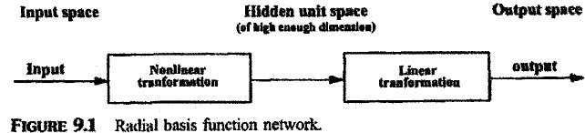
As mentioned, the RBF method is developed from the exact interpolation approach, but with modifications, to provide a smooth interpolating function. The construction of a radial basis function network involves three different layers, namely, an input layer, a hidden layer, and an output layer. The input layer is primarily made up of source nodes (or sensory units) to hold the input data for processing. For an RBF in its basic form, there is only one hidden layer. This hidden layer is of high enough dimensions. It provides a nonlinear transformation from the input space. The output layer, which gives the network response to an activation pattern applied to the input layer, provides a linear transformation from the hidden unit space to the output space. Figure 9.1 shows the transformations imposed on the input vector by each layer of the RBF network.

It can be noted that a nonlinear mapping is used to transform a nonlinearly separable classifica¬tion problem into a linearly separable one.
As shown in Figure 9.1, the training procedure can then be split into two stages. The first stage is a nonlinear transformation. In this stage a nonlinear mapping function of high enough dimensions is to be found such that we will have linear separability in the space. This is similar to what we discussed on the machine in Chapter 3, where a non-linear quadratic discriminant function is transformed into a linear function of f_i(x), i = 1,..,M, representing, respectively, and are linearly independent, real- and single-value functions, which are independent of Wj (weight). Note that in this case the discriminant function d(x) is linear with respective to w_i but f_i(x) are not necessary assumed to be linear.
Let us come back to the radial basis function problem. The basis functions used in this scheme are all localized functions. The parameters governing the basis functions (corresponding to hidden units) can be determined by using relatively fast, unsupervised methods. Some of these methods were discussed in Chapter 6. In these methods, only the input data are used. The second stage of the RBF network (i.e., from the hidden unit space to the output space) is a linear transformation that determines the weights for the final layer. It is a linear problem and is therefore fast also.
As mentioned in the previous paragraph, a radial basis function network is a modification to the exact interpolation approach, in which the number of basis functions is determined by the complexity of the mapping to be represented rather than by the size of the data set. That is, the number of the basis functions is much less than that of the pattern data points (M«N where M is the number of basis functions and N represents the number of pattern data points). With such an argument, the centers of the basis functions will not be constrained to the input data vectors. Suitable centers will be determined during the training process. Let x be a d-dimensional input vector, t a target vector which is one-dimensional, N the number of input vectors xⁿ, n= 1,2,...N, and M the number of basis functions in the hidden unit. A set of basis functions can be chosen with the following general forms: . The argument of the function is the euclidean distance of the input vector x from a center c_i. This justifies the name radial basis function.