"An introduction to genetic algorithms for scientists and engineers"
David A. Coley
Chapter 4, 59-67p.
4.1 Advanced Operators.
Although simple genetic algorithms, such as LGA, can be used to solve some problems, there are numerous extensions to the algorithm which have been developed to help improve performance and extend the range of applicability. These include more efficient crossover and selection methods, algorithms that deliberately hunt for local optima, combinatorial optimisation techniques, techniques to deal with multicriteria problems, and hybrid algorithms which combine the speed of traditional search techniques with the robustness of GAs. Being an introductory text, many of these extensions can not be given full justice and can only be outlined. For additional details, readers are directed to other texts, in particular references [MI94, ZA97 and BA96]. In addition, some of the techniques are described in more detail and then applied to various problems in Chapter 6.
Combinatorial Optimisation
Many problems do not require the optimisation of a series of real-valued parameters, but the discovery of an ideal ordered list, the classic example being the Travelling Salesman Problem (TSP). In the TSP a fictitious salesperson is imagined having to find the shortest route, or tour, between a series of cities. Typically the rules state that no city is visited more than once. Other examples of such combinatorial problems are gas and water pipe placement, structural design, job-shop scheduling, and time tabling.
A great deal of effort has been applied to trying to find efficient algorithms for solving such problems and this work has continued with the introduction of GAs. The main problem with applying a genetic algorithm, as described so far, to such a problem is that crossover and mutation have the potential to create unfeasible tours. To see why this is, consider the TSP described by Figure 4.1. Here there are eight cities, labelled a to h, arranged randomly on a plane. Table 4.1 lists the relative distances between each city.
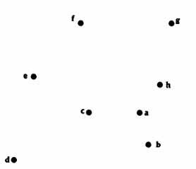
Figure 4.1. A TSP. What is the shortest tour that connects all eight cities?
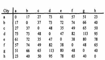
Table 4.1. Distance in km between the cities in Figure 4.1.
One example of a tour might be, b c de ghfa, another , c b gfa de h. If single-point crossover is applied directly to these tours the result, cutting at the mid-point, is : b c de adef and c b gfg hfa. Neither of these represents a complete tour.
So, how can a crossover operator be designed that only generates complete tours? If the strings used to represent the tours are to remain of fixed length, then this also implies that each city can only be visited once. There are many ways of constructing such an operator. One would be to apply crossover as before, then reject any incomplete tours generated. However, this would require rejecting most tours and it is relatively easy to imagine far less wasteful algorithms. One possibility is Partially Matched Crossover(PMX).
The TSP representation described above gives the strings a very different property to the strings used to respect real-valued optimisation problems. The position and value of an element are not unrelated. In fact, within the TSP it is only the order which matters. Ideally, the new crossover and mutation operators must not only create feasible tours but also be able to combine building blocks from parents of above average fitness to produce even fitter tours.
PMX proceeds in a simple manner: parents are selected as before; two crossover sites are chosen at random (defining the matching section) then exchange operators are applied to build the two new child strings.
Returning to the previously defined tours, and selecting two cut points at random: tour 1=bc/deg/hfa and tour 2 = c b / gfa/deh. First the whole centre portion or matching section is swapped: tour 1' = bc/gfa/hfa and 2' = cb/deg/deh.
Neither of these tours is a feasible tour. In tour 1' there is no d or e and in tour 2' cities a and f are not visited. As the strings are of fixed length, this means that both tours visit some cities more than once. In the case of tour 1' cities a and f are visited twice, tour 2' visits d and e twice. By definition, one of these repeats is within the matching section and one without. Also by definition, any city that is visited twice by one tour must be missing from the other tour. This suggests a way forward. Cities that are visited twice in one tour are swapped with cities that are visited twice in the other tour. Only one representative (the one not in the matching section) of such cities is swapped—otherwise the process would be circular and unconstructive. So, in this example, a outside the matching section of tour 1' swaps with the d of tour 2', and similarly for the cities f and the e. The two tours: tour 1" = bcgfahed and tour 2"= cbdegafh are formed, each of which is complete.
PMX is relatively easy to implement within LGA by making suitable alterations to the crossover operator and setting Pm to zero.
4.2 Locating Alternative Solutions Using Niches and Species.
In most optimisation problems the hunt is for the best possible solution. This might be the global optimum if this can be found, or a point in the vicinity of the global optimum if the problem is very large and difficult. However some problems are characterised by a search for a series of options rather than a unique solution vector. Problems in which these options reside at some distance from the global optimum are particularly interesting. In such cases there is a likelihood that the options are separated by regions which equate to much poorer solutions; rather than trying to avoid local optima, the idea is to try and hunt them down. Such a fitness landscape is illustrated by the multimodal function f(x) shown in Figure 4.2. Although intuitively there is something distinctive about the values of x which equate with peaks in f(x), mathematically none of them gives rise to a fitness greater than many of the points near the global optima. This begs the question, why hunt specifically for such values of x if any point near the global optimum is likely to generate higher fitness anyway?
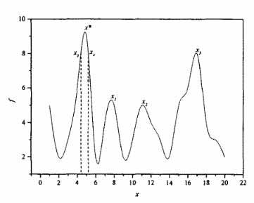
Figure 4.2. A multimodal function with a global optimum at x* and secondary, or local optima, at x1, x2 and x3.
One reason for attempting such searches can be best explained by an example. If the problem characterised by the fitness landscape shown in Figure 4.2 was an architectural one, in which x was the angle of a pitched roof and f the inverse of the financial cost of the construction, then each local optima take on a significant meaning. They represent good, but not ideal, financial solutions of radically different form. If cost is the only criterion, then angle x* is the only choice; however if any of the solutions x1, x2 or x3 are deemed to be more in keeping with other, visual, desires then the architect might be able to convince the client to invest the small amount of extra capital required. Although there are many points close to the global optimum that offer better values of f than any of the local optima, their closeness to the global optimum may produce little justification for adopting such a design rather than the optimum. This is not so for those structures represented by the local optima. In essence, the optimiser is being used as a filter, a filter charged with the task of finding highly performing, novel solutions to the problem across the whole problem space and ignoring, as much as possible, all other points. One way of finding such optima is simply by the use of multiple runs.
If all optima have equal likelihood of being discovered then R should be set by: R = p (0.577 + log p), where p is the number of optima. As all optima will not generally be equally likely to be discovered, R will typically need to be much greater than this. Figure 4.3 shows a more complex search space. The quest is for a technique that can effectively filter out any points that generate a fitness less than some minimum fmin. Such a filter would, if perfect, generate Figure 4.4, which is much easier to interpret than the original function. In the figures shown, this filtering is easy to apply by hand because the value of f is known at every point (x,y) within the problem space. Ordinarily f is likely to be far too complex to be estimated at more than a small fraction of the search space. So a technique is needed that can hunt for peaks within a complex landscape. This is somewhat ironic; up until now the central consideration has been the avoidance of local optima, now the desire is to actively seek them.
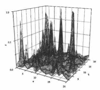
Figure 4.3. A more complex multi-peaked landscape; points of interest are those with f>fmin
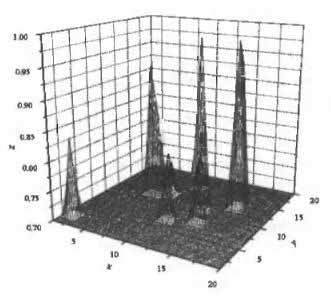
Figure 4.4. A filter version of figure 4.3 showing only points with f>fmin
In nature the exploration of separate fractions of the search space (or niches) by subsets of the population (or species) occurs readily. In applying this to the GA, the two most important concepts turn out to be fitness sharing and restrictions on who can mate with whom. That mating has to be restricted to closely related strings is not altogether surprising, it is after all one of the definitions of a species. That sharing the fitness between strings is important is more surprising.