The problem of definition of laws of distribution of processes on an exit of dynamic model of EMC is considered. Depending on volume of the initial information it is recommended to use Johnson's laws, Pirson's laws or beta-and gamma-distributions. Results provide reliability of an estimation EMC.

Problem definition. Evaluation of electromagnetic compatibility (EMC) is carried out in two stages: first is the reaction of y(f) object on the pullback, and then - EMC performance [1]. At the first stage there is no difficulty, because the reaction and the hindrance are connected with linear differential equation. At the second stage problem is nonlinear, because for capacity reaction calculation it is necessary to bring the reaction squared.

Effects of process z=y²(t) cannot be found instantly, so it is necessary to take into account the inertance of the object. It is realized by the a square pass through the inertial reaction or link, or through the window Diryhle. In the first case the link is established by time T, which coincides with the permanent inertia object. At the exit link flows quadratic inertial process (QIP) w_T(f). Such «inert» principle is adopted in standardized doses flikera voltage [2, 3], where T = 0.3 s. In the second case the current averaging of process runs z(f) at a given interval. This approach is used in [3] standardized deviations and frequency deviations unsymmetry and unsinusoidality voltage (wide range - from 3 to 60 s).

For abridgement further is considered only QIP, but all conclusions are distributed to the quadratic cumulative processes. The problem is in determining of the calculated maximum w_Tmax and minimum w_Tmin QIP with integral probabilities E_x and 1 - E_x(in [3]E_x = 0.05). You need to define the laws of probability distribution QIP.

The exact solution of the problem is known only obstacle in the form of a periodic sequence of rectangular pulses, and the telegraph signal [1]. In other cases, only moments of probability distributions can be determined [4, 5].

In practice the reaction is usually a stationary random process with normal distribution ordinate. The purpose of the article is to develop approximate methods of evaluation design extreme QIP for such processes.

Using series. In [5] the density distribution is recommended to approximate by Edzhuort number - by formula (34.15), using average w_T, skewnessS_kT and kurtosis E_hT. With considering correlation [6, 7] :

Ф_Фⁿ⁺¹=(-1)ⁿФ_Ф^'(x)H_n(x), Ф_Ф^'(x)=φ_Ф(x), H₀(x)=1,

H_n+1(x)=xH_n(x)-nH_n-1(x), n=0,1,...,

write it as a

where Hn (x) - polynomial Ermita, and П_w=(w_T-w_Tn)/σ_w Ф_Ф(x) and φ_Ф(x) - is a function and density of the standard normal distribution with zero mean and unit standard.

Let’s show the application of this series for example, when the exact solution is known: at T = 0 when QIP coincides with z (f). First consider the case when the average y_c of all responses is zero, which is typical for a dose flicker and unsinusoidality voltage. In this case formula (2.39) [1] gives the density

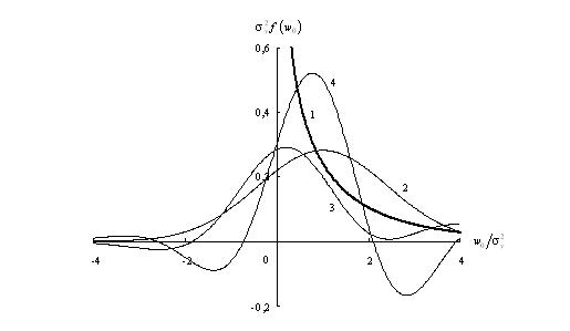
where w0 = z, σ_y - the reaction standard. The graph of density distribution is presented in Fig. 1 by the curve 1, where the axis of coordinates are taken in relative units.

With general formulas of probability theory we will determine numerical characteristics of distribution: w_n=σ_y², σ_no=√2σ_y², Sk_no=2√2, Ex_no=12 as well as second m_n2=3σ_y⁴ and thirdm_n3=8σ_y⁴ initial points. If we take only the first two characteristics, the formula (1) remains the first plugin, so the distribution is normal (curve 2). Consideration is also asymmetry, or asymmetry and kurtosis gives density graphs that are presented by curves 3 and 4.

Calculations show that even at high steady-time curves of the densities are very large areas of negative abscissa and the ordinate (Fig. 27 in [5]). This contradicts to the physical sense, that is why Edzhuort number is unacceptable.

Now for the approximation of the density distribution of Laguerre series, which typically use three numerical characteristics [6].

Denote

η=w_n²/σ_wT², λ=w_n/σ_wT²

where Г(x) - gamma function, x - argument.

Zero member generalized Laguerre polynomial is equal to one, and the third is

L₃(x)=1/6[η(η+1)(η+2)-3x(η+1)(η+2)+3x²(η+2)-x³] where η>0

The searched density distribution is:

If b3 = 0 formula (4) gives the gamma distribution

with parameters (3). In particular, for example, which is considered, we have η=0.5, λ=σ_y², b₀=1/√π, b₃=0 that is why the formula (4) coincides with (2) and (5), ie in this case gives the exact number of Laguerre solution (curve 1).

The change of densities in species in the growth of sustainable we will show on the example of reactions with zero mean and exponential α. At T = 0 curve 1 (Fig. 1 and 2) has an correlation function with parameter infinite ordinate and decreases monotonously, while T> 0 density curves start from scratch and have at least one maximum. Sustained increase in time reduces the range of change abscissa increases first maximum (curves 2 and 3). When αТ = 10 the curve 3 is almost symmetrical, but it is different from the normal distribution curve, since its maximum offset left of the mean value w_n/σ_y²=1 As for gamma distribution it can be considered that the normalization is at αТ>= 30 [8]

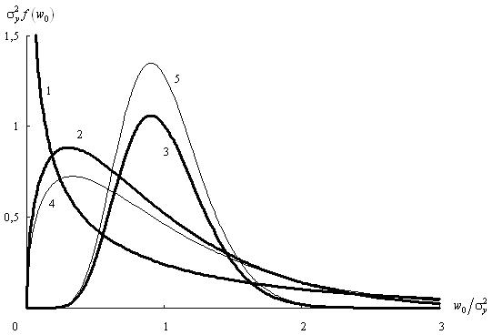
The densities can have negative ordinate, but they are much smaller in comparison with several Edzhuort. For example, curve 2 in Fig. 2 with absciss 4 has ordinate -0.00083. In this circumstances the application of Laguerre series is more correct.

For comparison 2 curves 4 and 5 aligned in the Figure 2, that related to the gamma distribution (at b₃ = 0). Each of them has a maximum and a positive ordinate.

For the case when the average response value is different from zero (for example, voltages unbalance). There is the exact solution formula :

where a=y_n/σ_y is a return value of the variation coefficient. At у_с = 0 the expressions (2) and (6) are coincided.

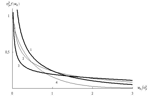
Curve 1 in Fig. 3 refers to a = 0, and therefore coincides with the curves 1 in previous figures. Curve 3 is calculated by formula (6) at -1=а=1. Apparently, the presence of nonzero average does not change species density curve, but it makes the extinction in the zone of large abscissa slower and in the zone of small abscissa - the opposite.

Curves 4 and 2 represent the approximate solution: a Laguerre series (4) and gamma distribution (5). They are located also differently relative to the curve 1. This leads to significant differences in calculated maximum, so there is unacceptable to neglect by value b₃ in (4) is unacceptable.

In all cases the average value is equal to the square of reaction effective value

w_n=y_a²=y_n²+σ_y² (7)

For the exponential correlation function reaction the standard is calculated by analogy formula (4.55) in [1]:

where D₁=2σ_y⁴, D₂=4y_n²σ_y² – plugins of variance square reactions. Distribution function F(w_T) is determined by the density, to find the calculated minimum and maximum from the equations:

Using the density distribution. Choice of the QIP law distribution depends on the amount of initial information. If you know there are four primary points, it is natural to use four parametric Pearson and Johnson distributions [8]. Unknown parameters of distribution, including range (w_Tm, w_TM) of possible values ordinate, is calculated by numerical methods of moments. In many cases, you can take w_Tm = 0, that allow to use the law of three parametric distribution.

If the range is known, it is enough to know average w_с and standard σw_T. In this case it is advisable to use a beta distribution by the density

where γ and η – parameters, κ =w_TM-w_Tm – range width, В(γ,η) – beta-function. At

parameters

Difficulties in defining of the parameters are needed to develop the simple oriented methods. At low average meanings (up to 10% of σ_у ) we are proposed to accept gamma distribution (5). This possibility is owing to the following. At T = 0, when the skewness and kurtosis are the largest, this distribution gives the exact solution. A small error would be at very large and steady time. In intermediate cases, at the important area of accounting for the density maximum the meanings (4) and (5) differ little. Gamma distribution does not give irregular fluctuations and negative ordinate. Decisive positive quality is that the gamma distribution requires a minimum amount of information: only the average value and standard that is defined by the average values and correlation functions of the reaction.

When large average meanings can be used Laguerre row but only to calculate the largest possible value w_TM of QIP ordinates. For this in the second equation (9) there is necessary to substitute the boundary probability 0001, that is considered the lowest meaning in practice at the determining of expected value w_TM > w_Tmax. The lowest possible value wTM is made equal to zero. The searched density is approximated by beta distribution, with parameters, except of w_Tm and w_TM, that are determined by formulas (11). Extremums calculations are received by the interpretation of equations (9).

Conclusions.

1. Edzhuort row using to determine the density distribution of quadratic inertial ordinate and cumulative processes is incorrect.

2. Distribution density worthwhile to approximate by divisions of Johnson and Pearson - with four points of known distribution, gamma distribution - in the first two points of distribution and low average values of reactions, the beta distribution - with major averages to determine the most possible value of Laguerre row with the boundary probability 0001 .

1. Кузнецов В. Г., Куренный Э. Г., Лютый А. П. Электромагнитная совместимость. Несимметрия и несинусоидальность напряжения. – Донецк: Норд-Пресс, 2005. – 250 с.

2. CEI/IEC 61000-4-15. Electromagnetic compatibility – Part 4, Section 15: Flickermeter – Functional and design specification. 1997.

3. ГОСТ 13109-97. Межгосударственный стандарт. Электрическая энергия. Электромагнитная совместимость технических средств. Нормы качества электрической энергии в системах электроснабжения общего назначения. – Введ. в Украине с 01.01.2000.

4. Васильев Д.В. Инерционное детектирование случайной последовательности прямоугольных импульсов. – Изв. вузов. Радиофизика, 1960. – С. 1011-1021.

5. Свешников А.А. Прикладные методы теории случайных функций. – М.: Наука, 1986. – 463 с.

6. Тихонов В.И., Статистическая радиотехника. – М.: Сов. радио, 1966. – 678 с.

7. Математический анализ: Функции, пределы, ряды, цепные дроби / Под общ. Ред. Л.А. Люстерника, А.Р. Ямпольского. – М.: Физматгиз, 1961. – 439 с.

8. Плескунин В.И., Воронина Д.Е. Теоретические основы организации и анализа выборочных данных в эксперименте. – Л.: изд-во Ленинградского ун-та, 1979. – 232 с.