1. Introduction

Because of the uncertainties in the numerical weather prediction (NWP) models, analyses, and forecasts, ensemble methods have been studied in the research community quite extensively in recent years. Many forecast centers around the world, such as the European Centre for Medium-Range Weather Forecasts (ECMWF) and the National Centers for Environmental Prediction (NCEP), have also developed and implemented various ensemble forecast systems to generate forecast references and guidelines in addition to the deterministic ones. The short-range ensemble forecasts (SREFs) concern forecast lead times between 0 and 48 h, and typically use limited-area models with relatively fine spatial resolutions and frequent forecast outputs. With the advance of computational ability and the success of the medium-range ensemble forecasting, Brooks et al. (1995) examined the feasibility of SREF applications in NWP. Du et al. (1997) examined the impact of initial condition uncertainty on quantitative precipitation forecasts from SREFs based on a mesoscale model. Hamill and Colucci (1997, 1998) evaluated the performance of National Oceanic and Atmospheric Administration (NOAA)/NCEP’s Eta Model–Regional Spectral Model (RSM) SREFs. Following these studies, an experimental SREF was developed at NOAA/NCEP, and a series of studies were conducted for evaluating this system (e.g., Stensrud et al. 1999;Wandishin et al. 2001). The further development of this system into operations has been described in Du and Tracton (2001), and the possibility of including members from the NOAA Rapid Update Cycle (RUC) forecast system has been reported upon in Lu et al. (2004). A comprehensive verification of SREF was also conducted in Hou et al. (2001) for the Storm and Mesoscale Ensemble Experiment (SAMEX).

The NOAA RUC forecast system (Benjamin et al. 2004a,b; Bleck and Benjamin 1993) has been consistently putting out regional weather forecasts in the short range over the years. Because the RUC system assimilates high-frequency observational data in an hourly cycle, its 1–12-h forecasts have provided a valuable reference and complement to less frequently updated forecasts from other operational NOAA models. Also, because of the same reason, one may wonder how forecasts from these hourly initializations vary, and, if there is some variability, how feasible and sensible an ensemble forecast is by using these forecasts as a set of ensemble members.

Time-lagged ensemble forecasting has been studied and proposed for the medium range of 6–10 days (Hoffman and Kalnay 1983; Dalcher et al. 1988; van den Dool and Rukhovets 1994). The concept has also been applied to the short-range forecast recently in Hou et al. (2001) and in Walser et al. (2004). We have experimented with the time-lagged ensemble approach using the NOAA RUC for a number of years. The current study is a report on this effort. We believe that the method we present in this study can be applied to any rapid update data assimilation and forecast system.

One reason to adopt the time-lagged ensemble technique to the short-range forecasting is because a shortrange forecast generally possesses a relatively strong dependency on the initial conditions. The forecast errors in the very short range may be strongly correlated to the uncertainties in the initial analysis. The timelagged ensembles can be interpreted as forecasts obtained from a set of perturbed initial conditions (van den Dool and Rukhovets 1994). Because these initial perturbations are generated from different forecast initialization cycles, conceptually, time-lagged ensembles reflect the forecast error covariance with time-evolving (flow dependent) information. In the very short range, this flow-dependent forecast error can be, for example, a result of an initial imbalance or a shock of model fields due to various data being ingested at initialization time and the ensuing adjustment of the model fields.

In this study, we will report on how a time-lagged ensemble forecast system can be constructed using forecasts from the RUC, and evaluate how much skill this type of ensemble forecast can provide over each individual deterministic forecast for the very short range weather prediction of 1–3 h. This type of shortrange ensemble forecast system could be used in shortrange decision support systems, such as those for aviation weather forecast applications including air traffic management, in which case frequent updates to a forecast are needed. Analyses and verification of these time-lagged ensemble systems, for both the ensemble mean and probabilistic forecasts, will be conducted. We will introduce two different approaches for the weighting of RUC hourly forecasts, and compare the improvement of short-range forecasts by these two ensemble systems.

The paper is organized as follows. In section 2, we will first give a brief description of the NOAA RUC data assimilation and modeling system. We will then examine the forecast variability among forecasts from different initialization cycles. Next, we will describe how to construct time-lagged ensembles using the eight available deterministic forecasts within a 12-h initialization cycle, and briefly introduce the verification– observation data and method. In the next section, we obtain time-lagged ensemble forecasts using a simple ensemble mean approach (equally weighted). These time-lagged ensembles along with various deterministic forecasts are verified against upper-air (rawinsonde) observations at station locations (section 3). To further reduce the ensemble forecast error, we construct timelagged ensembles with unequal-weighted forecasts using a multilinear regression method (section 4). Conclusions will be provided in section 5.

2. Time-lagged ensemble method

a. Description of the forecast model

The NOAA RUC forecast/data assimilation system was developed at the NOAA/Forecast Systems Laboratory (currently, the NOAA/Earth System Research Laboratory/Global System Division), and has been used as the operational forecast model for the Federal Aviation Administration (FAA) and also been used as the rapid update forecast and data assimilation system at NOAA/NCEP. The model’s dynamical core is composed of a hybrid terrain-following sigma (at lower levels) and isentropic (at upper levels) vertical coordinates, and a set of hydrostatic primitive equations. In addition, there is a complete set of physical parameterization schemes, including those for the planetary boundary layer, radiation, land surface physics, cumulus convection, and explicit mixed-phase cloud physics, to represent various physical processes in the model and to close the model dynamic equations. The data assimilation system includes a series of implementations of optimal interpolation (OI), three-dimensional variational data assimilation (3DVAR) analysis, and the nudging technique. The nudging technique is mostly applied to the surface fields, while the main atmospheric fields are assimilated with the 3DVAR algorithm. The lateral-boundary conditions are given by NCEP Eta Model (for detail, see the aforementioned references).

The RUC horizontal domain covers the contiguous United States and adjacent areas of Canada, Mexico, and the Pacific and Atlantic Oceans. The operational RUC has been run at a series of horizontal grid spacings: 60, 40, 20, and 13 km. In this study, we use the 40-km resolution analyses and forecasts during November and December of 2003. There are 24 runs per day, but we only use the forecasts that are initialized within 12 h previously. The hourly runs of the operational RUC 40-km data are archived for only the first 6 h, with the longer archives limited to the 3-hourly runs (e.g., 0000, 0300, 0600 UTC, etc.).

b. Variability in the RUC hourly forecasts

To examine the variability of the hourly initialized RUC forecasts, we randomly picked a case from the archive of RUC operational forecasts during the winter season of 2003/04. The case constitutes forecasts valid for 0000 UTC 15 December 2003, and initialized, respectively, at 12, 9, 6, 3, 2, and 1 h prior to the initial times. In this case, there were two winter synoptic weather systems most evident in these forecasts: a cutoff low pressure system along the United States east coast, situated over the New England states, and a deep low pressure trough extending from central Canada into the central United States, with strong cold-air advection of an arctic air mass behind this trough from western Canada into the western high plains and western United States.

While the forecasts present consistent big pictures of the geopotential height field, there are some disagreements on the depth (intensity) of the two synoptic systems. In particular, the older the forecast is, the larger is the difference with reference to the 1-h forecast. The 12-h forecast predicted a deeper 850-hPa low with a somewhat stronger cold-air surge in the vicinity of Lake Winnipeg in Manitoba, Canada. These differences in large-scale geopotential height field will evidently result in different upward–downward air motions of winter storms associated with these two weather systems. The associated upward and downward motions indeed demonstrate some disagreements here and there, especially in association with the two synoptic-low systems.

c. Construction of the time-lagged ensemble system

Because we are interested in the short-range ensemble forecasting, only deterministic forecasts within a 12-h cycle (previous forecasts up to 12 h) are considered for the ensemble member pool. Figure 3 shows schematically a time-lagged ensemble forecast system. Because the forecast data from the hourly initialization for operational 40-km RUC runs were archived up to 6 h, after that only the forecast data with 3-hourly initializations were archived, the maximum size of the timelagged ensembles that we could work with, within a 12-h cycle, is eight members (see Fig. 1). The timelagged ensemble is a single-model, initial-condition ensemble forecast system; that is, the model dynamics, physical parameterizations, and numerics are all the same. The differences among ensemble members come merely from different forecast projections or forecasts initialized at different times.

Figure 1 - Schematic diagram showing how a time-lagged ensemble forecast system is constructed.

In this study, we concentrate on the performance of time-lagged ensembles for the very short-range forecasts of 1–3 h. When the validation times are fixed, being 0000 and 1200 UTC (corresponding to the upperair observation times), the number of ensembles decreases by one member. Therefore, the maximum numbers of ensembles are eight, seven, and six for forecast lead times of 1, 2, and 3 h, respectively, given the RUC archive configuration. Figure 2 summarizes the available deterministic forecasts that are used to construct the time-lagged ensembles for the forecast verifications at 1-, 2-, and 3-h lead times.

d. Verification–observation data and method

The verification of forecasts (both deterministic and ensemble) was performed by interpolating RUC grid forecast fields to the rawinsonde observational sites, then comparing forecast values of state variables (height, temperature, relative humidity, and wind speed) against the observed ones, all at matching mandatory pressure levels (850, 700, 500, 400, 250, 200, and 150 hPa). The forecast errors (forecast-observed) were computed by assuming the observations represent the truth.

We used operational rawinsonde observations (twice daily), about 92 stations in the RUC model domain.

3. Equally weighted ensembles

a. Ensemble mean forecast

The simplest way to obtain an ensemble forecast is to take the arithmetic mean of values from the ensemble forecast members; that is,

(3.1)

where f^ and f_i, i=1,2,...,N, denote an ensemble forecast and N deterministic forecasts, respectively, and (x, t) denote spatial and time independent variables. The number of ensemble forecast members varies between 6 and 8, depending on a verification of a particular lead-time forecast (see pic. 2). Evidently, this ensemble forecast is obtained simply by weighting all member forecasts equally.

Figure 2 - Time-lagged ensemble systems for different forecast lead times defined by taking the RUC deterministic forecasts initialized at different analysis times.

b. Short-range forecast improvement

To examine how much improvement the time-lagged ensemble forecasts may provide, we first compute the skill scores of the mean absolute error using each deterministic forecast as a reference forecast. The skill score is defined (e.g., Wilks 1995) as

(3.2)

where A^=<|f^-f_T|> is an accuracy measure of an ensemble forecast, A_i=<|f^-f_T|> is an accuracy measure of a reference deterministic forecast, A_T=0 (here for the case of the observational errors not being accounted for), and f_T represents the verification "truth". The angle brackets represent a spatial and temporal average. The values f^ and f_i were defined previously in (3.1) with i=1,2,3 being the 1–3-h reference-forecast index (e.g., i=1 is for the 1-h forecast to be used as the reference forecast, and so on). Note that the reference forecast is always the most recent deterministic forecast. When all the forecast errors are taken as time- and domain-averaged values, the computed skill score will possess statistical robustness. In this study, we will compute skill scores averaged over all rawinsonde stations within the RUC model domain and over the winter period of November–December 2003.

In Figs. 3a–d, we plot the forecast skill scores of geopotential height, temperature, wind speed (determined by the magnitude of the horizontal wind vectors), and relative humidity at 850-, 500-, and 250-hPa pressure levels for the time-lagged ensembles with the deterministic forecasts of 1–3 h as the reference forecasts. One can see that in general, the ensemble forecasts have positive skill over the corresponding deterministic forecasts. The improvement in the forecasts ranges from a few percent to an order of 10%, depending on forecast variables and levels. It can be seen from these figures that the forecast improvement is generally smaller at upper levels and for wind fields. The improvements for the 1-, 2-, and 3-h forecasts are generally comparable. For the height field, there is slightly more improvement in the 1- and 2-h forecasts than in the 3-h forecast; while for temperature and wind speed, slightly more improvement is found in the 2- and 3-h forecasts than in the 1-h forecast. For relative humidity, a relatively significant improvement is found at the 500-hPa pressure level.

Figure 3 - Forecast skill scores provided by the time-lagged ensemble mean with 1–3-h RUC deterministic forecasts as reference, evaluated against rawinsonde observations ("truth") at three different pressure levels: 850, 500, and 250 hPa. The dark, medium, and light bars are for forecasts with lead times of 1, 2, and 3 h, respectively. Shown are the (a) geopotential height, (b) temperature, (c) horizontal wind, and (d) relative humidity.

The skill scores reflect an averaged improvement of the forecast over the entire domain covered by the rawinsonde observational sites. One may also want to know at how many sites this forecast improvement is actually realized. To answer this question, we evaluate the forecast error at each station and count the number of the stations at which the ensemble forecast has less error than does the deterministic forecast. In Figs. 4a and 4b, we plot the percentage of verification times at which the ensemble forecast is better than the deterministic forecast as vertical profiles for the 1-, 2-, and 3-h wind and temperature forecasts, respectively. We see that the percentage of the verification times for which the ensemble forecast performs better than the deterministic forecast is very high, and that this percentage decreases at higher levels (reaches a minimum at the 300-hPa pressure level for wind and 200-hPa level for temperature). This decrease in the percentage improvement at higher altitudes is consistent with the skill score calculation shown in Fig. 3. One of the explanations for the decrease of the skill at these levels is that the small smoothing effect provided by the ensemble means is overwhelmed by the large wind speed and large variation of temperature at the jet levels (200–300 hPa).

Figure 4 - Vertical profiles of the percentage of the total number of verification times the ensemble mean forecast was better than the deterministic forecast for RUC for the period November–December 2003 for the (a) horizontal wind forecasts and (b) temperature forecast.

c. Ensemble spread

To examine the spread of the time-lagged ensemble system, we plot the rank histogram (Talagrand diagram) for selected model fields from each verification category (1–3-h forecasts). The ranked histograms for the 1-, 2-, and 3-h lead-time forecasts are shown in Figs. 5a1–a3 for the geopotential height field at the 500-hPa pressure level, Figs. 5b1–b3 for the temperature field at the 850-hPa pressure level, Figs. 5c1–c3 for the wind field at the 250-hPa pressure level, and Figs. 5d1–d3 for the relative humidity at 850-hPa. One can see from these plots that the rank histograms generally displayed U-shaped distributions. This indicates that the timelagged ensembles constitute an underdispersive ensemble forecast system (Hamill 2001). There are a few factors that contribute to the small spread problem in the time-lagged ensemble system. First, the time-lagged ensemble forecast system is a single-model ensemble system: it does not account well for model error, which tends to give the largest ensemble spread. Second, the ensemble system is constructed directly from the forecasts with different forecast projections. Therefore, there is no breeding cycle (as in the NCEP method) and no maximization procedure (like the singular-vector method used in the ECMWF) for the "perturbations" to grow. Third, because all of the initialization times are so close to each other, the model dynamics will make all the difference among the ensemble members growing minimally (close to a linear fashion). Last, the small ensemble size reduces the ability of the ensemble to capture the full uncertainty in the forecast. Also indicated from these rank histograms is that slight biases are detected in all of the fields at various levels (because of the sloped distributions of the rank histograms toward one side). These biases are likely due to biases in the model background that feed the data assimilation, and then present themselves in the analysis cycle.

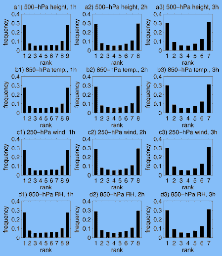
Figure 5 - Rank histogram for time-lagged RUC deterministic forecasts for the (a) 500-hPa geopotential height, (b) 850-hPa temperature, (c) 250-hPa wind speed, and (d) 850-hPa relative humidity, verified for forecast lead times of 1, 2, and 3 h.

d. Analysis of forecast improvement by the time-lagged ensembles

To understand why the time-lagged ensemble system improves short-range forecasts, we plot forecast error as a function of initialization time (Figs. 6a–d) for the following forecast variables at three different pressure levels: geopotential height, temperature, wind speed, and relative humidity. The forecast errors of the RUC deterministic forecasts initialized at 12, 9, 6, 5, 4, 3, 2, and 1 h prior are plotted as the thick solid curves, with asterisks used to mark their error sizes. Various types of lines represent forecast errors for time-lagged ensemble systems with three different forecast lead times (see fig. 2). Because there is only one value for each ensemble forecast error, either evaluated as a 1-, 2-, or 3-h forecast, there should be only one point represented in that error in this graph. However, we use horizontal lines to indicate these errors given by these ensemble systems. Note that the lengths of these lines vary, indicating different ensembles sizes of eight, seven, and six members, respectively, for 1-, 2-, and 3-h forecast lead times.

Figure 6 - Forecast errors in the (a) geopotential height, (b) temperature, (c) horizontal wind speed, and (d) relative humidity as functions of model initialization time. The solid curve with asterisks corresponds to deterministic forecasts from different forecast projections. Three different types of horizontal lines shown at the top right of each panel correspond to 1-, 2-, and 3-h forecasts from ensemble means (see Table 1), with error values horizontally extending back to indicate which deterministic forecast members were included.

Having explained how Figs. 6a–d were created, let us examine what these figures tell us. Figure 6c plots the forecast errors in the wind field. The error curve for the deterministic forecasts continuously comes down as the initialization time gets closer and closer to the verification time. This picture seems to fit the traditional thinking that an initialization with more recent data will produce a more accurate forecast. In this case, the improvement of the forecasts made by the ensembles seems to be minimal (or absolutely none, e.g., at the 250-hPa level for the 1-h forecast), which is consistent with Fig. 3c (only a few percent of skill or even negative skill). This minimal improvement in the forecast may be due to the ensemble average, which slightly reduces the model random errors. When examining Figs. 6a, 6b, and 6d, one can see that this picture is not always true. The forecast error associated with a deterministic forecast initialized farther back, such as -12 or -9 h, typically displays a larger error. This error typically decreases as the initialization moves closer to the verification time. However, when the initialization gets to the very short range of 1–3 h, the forecast error can increase again for certain forecast variables at certain levels. This phenomenon is customarily understood as the "model initial spinup" problem. There are two types of model spinup problems. One type results from the model internal diabatic physics trying to adjust to the nondiabatic initialization. This type of model spinup problem is usually reflected in the model convection and precipitation fields. Another type of model spinup arises because there exists a time period for the mass and wind fields to adjust to each other when ingesting wind- or mass-related observations into the model. Depending on the data type ingested and the scale of the weather feature, the spinup problem can occur on selected model state variables, either the mass or wind field. When these happen, for example, in the cases of the geopotential height and relative humidity fields at all levels in Figs. 8a and 8d, and in the case of the temperature at the 850- and 500-hPa levels in Figs. 6b1 and 6b2, a significant improvement by the ensemble forecast is more likely. Figures 3a and 3d also confirm this picture, where 10% or greater forecast skills can be achieved by the time-lagged ensemble system. The error analyses for the geopotential height, temperature, wind speed, and relative humidity in Figs

6a–d are consistent with our previous findings (Benjamin et al. 2004b, their Figs. 7a–c). Of course, the improvement of the forecast is also due to the smoothing effect of the ensemble mean, which tends to reduce the intense model features.

Figure 7 - The values of the DC component and weighting coefficients (for different deterministic forecasts) trained with November 2003 rawinsonde observational data using the multilinear regression algorithm.

4. Unequally weighted ensembles

a. The multilinear regression method

From the analysis in section 3, we know that the reasons why the time-lagged ensemble system improves the short-range forecast are that the average of the deterministic forecasts initialized at different times smoothes out the initial model shocks and that the ensemble mean tends to verify well because of the smoothing of the severe model features. However, the equally weighted ensemble approach presented above is evidently a crude way to obtain an ensemble forecast. We could further reduce the forecast error by choosing different weights for different forecast members according to their levels of imbalance. In doing so, we consider a multilinear regression method, similar to the method proposed by van den Dool and Rukhovets (1994).

Let us express an ensemble forecast as a weighted combination of deterministic forecasts; that is,

(4.1)

where b_i are N weighting coefficients for N forecast members and a denotes the DC (direct current: nonvariance) component for such an expansion. By requiring that a least squares error be achieved between the ensemble forecasts and the verification truth, one could get a set of linear equations for the set of regression coefficients:

(4.2)

where

(4.3)

and

(4.4)

are the covariance between the deterministic forecasts themselves, and the covariance between the verification truth and the deterministic forecasts, respectively. In (4.3) and (4.4), the computation of the covariance is taken over all verification data points k=1,2,...,K, and f_i and f_T are the expected values of the deterministic forecasts and the verification truth, respectively. We used one month’s data for the training period, and the other month’s data for the verification, and we also conducted a cross validation by switching the training and verification periods. The expect values in the above equations are obtained from the average of the entire training period.

Upon solving (4.2), one obtains a set of regression coefficients (weights) for each deterministic forecast used for the ensemble member. The DC component can be determined once b_i, i=1,2,...,N, are known:

(4.5)

An ensemble forecast system can then be constructed via (4.1) from these optimally determined weights.

We have developed a version of the RUC timelagged ensemble forecast system based on this multilinear regression method. Because the deterministic forecasts initialized at previous times and observations corresponding to these times all exist till the time of forecast, this algorithm could be implemented as a realtime ensemble forecast system.

b. Trained weights

Figures 7a–d plot the weighting coefficients as functions of the deterministic forecasts for height, temperature, wind speed, and relative humidity, respectively, at the 850-, 500-, and 250-hPa pressure levels. For the present case, the November 2003 rawinsonde data are used to train the RUC deterministic forecasts. The corrections for the DC component for these variables at various levels are indicated in the legend boxes as well. In general, the multilinear regression scheme tries to minimize the difference between the predictor and the predictand by achieving a balance among the DC component and all other variance components (weights). While the DC component provides a bias correction (variance independent), the weighting coefficients reflect the relative importance of each contributing member (forecast). The absolute value for each coefficient in Figs. 7a–d gives the weighting size of that forecast, while the positive or negative sign of an weighting coefficient for a particular forecast represents the weighting or counterweighting for the overall minimization.

One can see from Fig. 7c, in reference to Fig. 8c, that when the forecast error for wind decreases uniformly from the older to newer forecasts, the trained weighting coefficients corresponding to these forecasts do not possess a linear reduction of the weighting size. Instead, the training process tried to put almost all of the weighting to the most accurate forecast (initialized at the previous hour before the verification time), and assigned trivial weights to all other forecasts, but with alternating weighting and counterweighting (variations around the zero line). Clearly, the linear regression algorithm tries to deal with not only the model spinup error, but also other random model errors.

When the model initial spinup errors are most evident, for example, in the height and relative humidity fields (Figs. 6a and 6d), the weighting patterns are clearly diversified (Figs. 7a and 7d), in the sense that the 1-h forecast no longer possesses the dominant weight, but weights of similar magnitude can also be found variably with 2-, 3-, 4-, 5-, and even 12-h forecasts. The temperature at various levels in Fig. 6b is a case of a mixture of the two scenarios discussed above. Therefore, its weighting pattern (Fig. 7b) shows mixed features between the two opposite cases.

The overall trained pattern for the weighting coefficients is very similar for the use of December 2003 data, which is indicative of some level of reliability in the training results.

c. Verification of the unequally weighted ensemble forecasts

Cross validation was used to conduct an unequal weighting process for November and December by switching the training and verification months. We first compare the forecasts made by the equally weighted and unequally weighted ensemble systems for the period of November–December 2003. To do this, we compute the skill scores for the unequally weighted ensemble forecasts using the equally weighted ensembles as the reference forecasts. In this way, we can identify clearly the relative skillfulness between the two methods. Figures 8a–d plotted the skill scores for four forecast variables at three different pressure levels. One can see from these figures that the unequally weighted ensembles provided much better 1–3-h forecasts than do the equally weighted ensembles. For all variables and at all levels, the unequally weighted ensemble forecast displayed positive skills.

Figure 8 - Forecast skill scores for (a) geopotential height, (b) temperature, (c) wind, and (d) relative humidity for the unequally weighted ensemble system at the 850-, 500-, and 250-hPa pressure levels. The scores are calculated using the equally weighted ensembles as the reference forecasts for the forecast lead times of 1, 2, and 3 h.

To present this result in a bigger picture, we now plot the 1–3-h forecast errors for the deterministic and for two ensemble forecasts. In Figs. 9a–d, we plot the forecasts from the equally and unequally weighted ensemble systems to compare with that from the RUC deterministic forecast. It is seen from these figures that although the equally weighted ensembles improve the short-range forecasts in most cases in comparison with the deterministic forecasts, the ensembles using unequal weights make significant improvement over the deterministic forecasts for all variables at all levels. We should also point out that the error reductions shown in Fig. 9 appear to be small in the absolute sense, because these numbers are for a domain and a time average.

Figure 9 - Comparison of forecast errors for the equally weighted ensemble mean, unequally weighted ensemble mean, and deterministic forecasts for the (a) 500-hPa geopotential height, (b) 850- hPa temperature, (c) 250-hPa wind, and (d) 850-hPa relative humidity as functions of forecast time.

5. Conclusions

In this study, we have demonstrated how to construct a time-lagged ensemble system using the deterministic forecasts from a rapid updating forecast–data assimilation system, such as NOAA’s RUC model. Both equally weighted and unequally weighted methods have been used to combine these forecasts. Analyses and verifications of these ensemble-mean and probabilistic forecasts were conducted. The results can be summarized as follows.

1) The equally weighted ensemble-mean forecasts have some positive forecast skill over the deterministic forecasts for the short range of 1–3 h.

2) The ensemble systems composed of RUC deterministic forecasts are understandably underdispersive and also slightly biased.

3) From the analysis of the weighting coefficients, the improvement of the short-range forecasts by the time-lagged ensembles may be because the timelagged ensemble forecasts correct for forecast errors resulting from the model initial spinup.

4) Unequally weighed ensembles provide better ensemble systems. These ensemble systems result in a significant improvement over the deterministic forecasts in the short range of 1–3 h.

Acknowledgments. We thank John Brown, Kevin Brundage, and other NOAA/FSL RUC team members for discussions on the subject; Ligia Bernardit, who conducted the NOAA internal review; and Susan Carstan, who conducted the technical edit. This research was performed while H. Yuan held a National Research Council award at NOAA/ESRL. We also thank three anonymous reviewers for their constructive and helpful comments and suggestions, and Dr. David Stensrud for his excellent editorship for this work. This research is in response to requirements and funding by the Aviation Weather Research Program of the Federal Aviation Administration (FAA). The views expressed are those of the authors and do not necessarily represent the official policy or position of the FAA.

References

Benjamin, S. G., G. A. Grell, J. M. Brown, and T. G. Smirnova, 2004a: Mesoscale weather prediction with the RUC hybrid isentropic–terrain-following coordinate model. Mon. Wea. Rev., 132, 473–494.

——, and Coauthors, 2004b: An hourly assimilation–forecast cycle: The RUC. Mon. Wea. Rev., 132, 495–518.

Bleck, R., and S. G. Benjamin, 1993: Regional weather prediction with a model combining terrain-following and isentropic coordinates. Part I: Model description. Mon. Wea. Rev., 121, 1770–1785.

Brooks, H. E., M. S. Tracton, D. J. Stensrud, G. DiMego, and Z. Toth, 1995: Short-range ensemble forecasting: Report from a workshop, 25–27 July 1994. Bull. Amer. Meteor. Soc., 76, 1617–1624.

Dalcher, A., E. Kalnay, and R. N. Hoffman, 1988: Medium range lagged forecasts. Mon. Wea. Rev., 116, 402–416.

Du, J., and M. S. Tracton, 2001: Implementation of a real-time short-range ensemble forecasting system at NCEP: An update. Preprints, Ninth Conf. on Mesoscale Processes, Fort Lauderdale, FL, Amer. Meteor. Soc., 355–356.

——, S. L. Mullen, and F. Sanders, 1997: Short-range ensemble forecasting of quantitative precipitation. Mon. Wea. Rev., 125, 2427–2459.

Hamill, T. M., 2001: Interpretation of rank histograms for verifying ensemble forecasts. Mon. Wea. Rev., 129, 550–560.

——, and S. J. Colucci, 1997: Verification of Eta–RSM shortrange ensemble forecasts. Mon. Wea. Rev., 125, 1312–1327.

——, and ——, 1998: Evaluation of Eta–RSM ensemble probabilistic precipitation forecasts. Mon. Wea. Rev., 126, 711–724.

——, and J. Juras, 2007: Measuring forecast skill: Is it real skill or is it the varying climatology? Quart. J. Roy. Meteor. Soc., in press.

Hoffman, R. N., and E. Kalnay, 1983: Lagged average forecasting, an alternative to Monte Carlo forecasting. Tellus, 35A, 100– 118.

Hou, D., E. Kalnay, and K. K. Droegemeier, 2001: Objective verification of the SAMEX’ 98 ensemble forecasts. Mon. Wea. Rev., 129, 73–91.

Jolliffe, I. T., and D. B. Stephenson, 2003: Forecast Verification: A Practitioner’s Guide in Atmospheric Science. John Wiley and Sons, 240 pp.

Lu, C., S. G. Benjamin, J. Du, and S. Tracton, 2004: RUC Short-Range Ensemble Forecast System. Preprints, 20th Conf. on Weather Analysis and Forecasting, Seattle, WA, Amer. Meteor. Soc., CD-ROM, J11.6.

Stanski, H. R., L. J. Wilson, and W. R. Burrows, 1989: Survey of common verification methods in meteorology. WMO World Weather Watch Tech. Rep. 8, 114 pp.

Stensrud, D. J., H. E. Brooks, J. Du, M. S. Tracton, and E. Rogers, 1999: Using ensembles for short-range forecasting. Mon. Wea. Rev., 127, 433–446.

van den Dool, H. M., and L. Rukhovets, 1994: On the weights for an ensemble-averaged 6–10-day forecast. Wea. Forecasting, 9, 457–465.

Walser, A., D. Luthi, and C. Schar, 2004: Predictability of precipitation in a cloud-resolving model. Mon. Wea. Rev., 132, 560–577.

Wandishin, M. S., S. L. Mullen, D. J. Stensrud, and H. E. Brooks, 2001: Evaluation of a short-range multimodel ensemble system. Mon. Wea. Rev., 129, 729–747.

Wilks, D. S., 1995: Statistical Methods in the Atmospheric Sciences:An Introduction. Academic Press, 467 pp.

Wilson, L. J., 2000: Comments on “Probabilistic predictions of precipitation using the ECMWF Ensemble Prediction System.” Wea. Forecasting, 15, 361–364.