
Introduction
1. The object and purpose of the study
2. Objectives
3. Methods of forecasting of arterial pressure
4. Algorithm for data preprocessing
Conclusion
List of used literature
Cardiovascular diseases are a major cause of mortality worldwide. On average one in three people die from diseases of the circulatory system. To prevent them to study hemodynamic assessment of the impact of various influences on the body, etc. To this end, A numerical model of the circulatory system.
Among the most dangerous situations that occur in intensive care wards, are episodes of acute hypotension, which require an effective surgical intervention..
Arterial hypotension (hypotension) is a condition characterized by persistent lowering of blood pressure. There are physiological and pathological arterial hypotension (acute and chronic). Severe hypotension develops acute cardiovascular or circulatory collapse, with shock of various origins and collapse, with significant blood loss, intoxications and infectious diseases, with severe sickness syndrome, and in certain other pathological conditions of the organism. Chronic pathological arterial hypotension is the primary (essential) and secondary (symptomatic).
Primary chronic hypotension depends on the dysfunction of higher centers of autonomic vasomotor regulation in connection with which there is an infringement of vascular tone (dysfunction of the nervous system and humoral) in violation of the microcirculation, capillary permeability and in violation of the rheological properties of blood.
Secondary chronic hypotension depends on a basic pathological process, which determines the low blood pressure. Clinical symptoms: on the background of a constitutionally or genetically caused vegetative-vascular dystonia as a possible increase in blood pressure and its reduction.
If untreated, episodes of acute arterial hypotension may lead to irreversible organ damage and death. Timely and appropriate measures can reduce these risks, but the wrong measures may be ineffective or even dangerous. The definition of what intervention is appropriate in each case depends on a correct diagnosis of the causes of the episode, which may be sepsis, myocardial infarction, cardiac arrhythmia, pulmonary embolism, hemorrhage, dehydration, anaphylaxis, the influence of drugs, or any of a wide range of other causes of hypovolemia, vazodilyatornogo heart failure or shock. Often the best choice may be suboptimal, but relatively harmless intervention, merely in order to gain enough time to select a more effective treatment without subjecting the patient to additional risks.
Approximately one-third of ICU patients with reported cases of severe hypotension. The mortality rate for these patients in more than two times higher than other patients. Therefore, prediction of what can be expected episodes of acute hypotension, would create an opportunity to improve care and increase the probability of survival of patients with the occurrence of these episodes.
The purpose of my Master's work is to develop an information system to predict which patients will experience an acute episode of hypotension during the early hours after the current time in time series of basic health indicators.
Initial data for time series prediction are mean arterial pressure (ABP) at minute intervals. Each record of the time series is mean arterial pressure measured at the radial artery in a minute. For these time series data necessary to identify those patients who will be observed episodes of acute hypotension. Episodes of acute hypotension assume any period of 30 minutes or longer during which at least 90% of all measurements of mean arterial pressure did not rise above 60 mm Hg.
To test the system under development are taken data from the database MIMIC II Database [1] which contains information on 30,000 patients with ICU care.
Entries MIMIC II Database contains much information which may appear in medical records, as well as signals that are available for observation by members of the ICU. In other words MIMIC II Database is sufficiently detailed for use in research that might require access to intensive care. Therefore, this database is a good source of information for the development and evaluation of diagnostic and prognostic algorithms, and in particular to address the problem of my master's thesis.
3. Methods of forecasting of arterial pressure
3.1 Models of the cardiovascular system of man
Modern "reservoir" ( "compartments") model of the cardiovascular system of man (SSSCH) initiated, as is known, the model of Otto Frank, published in the late 19 th century. Frank proposed to represent the aorta as an elastic reservoir, acting as a hemodynamic "damper" systolic blood flow from the left ventricle of the heart. Theoretical studies of reservoir models SSSCH become popular since the mid 20 th century and focused on the development of biological concepts of the theory of regulation. However, applications of this theory were limited to identifying relationships between the average ( "minute") values of pressures and flows. Therefore, in particular, there is no theory of relationships end systolic pressure (SDC) to the end-diastolic pressure (CRT), which is widely used in medical diagnosis.
3.1.1 The one-part model
The simplest model of the aorta and major arteries in the form of a general elastic reservoir ( "chamber") is analytically given by a system of three linear equations:
According to these equations, 1) the rate of change "active" volume of the chamber du / dt is equal to the difference between the input f
System (1), containing a single linear differential equation and two linear algebraic equations, allows the selection of one ordinary differential equation (ODE) with respect to the variable pressure p (t):
Where α= 1/rc 1/ / is time factor and the reciprocal of τ - «time constant».
In the model of Frank's blood is the source of input f0(t) given as a periodic function of time. Rectangular pulses described by the function:
in formula (1) the brackets denote the function "integer part", 2 nd formula determines the value of U in the stroke volume of blood. Some authors represent systolic flow pulses parabolic shape, then instead of (3) have a flow:
Let the initial time p(0) ≡ p0 known end-diastolic pressure (ESP), and p(T1) ≡ p1 unknown end systolic pressure (ESP). Then, solving the ODE (2) for pulse flows (3) and (4), we get a couple of functions that describe the change in pressure in the adjacent phases of systole and diastole,
t ∈[T1; T]: p(T)= pd(t)= p1 exp( -α(t-T1))+ P exp(- α(t-T1)); (5b)
where Exp(t) 1 - exp(t), and the function F (t) - contribution of the systolic pulse, which for a rectangular pulse and a parabolic form is defined, respectively, as follows:
Piecewise Exponential description of the two phases of relaxation oscillations of pressure provided by a pair of functions (5a) and (5b), belong to the same cycle. In order to obtain high cycle description of these fluctuations, suitable for algorithmic (computer) charting, you should use the above-introduced "sawtooth" function of time θ(t), augmented by two logical implication:
From the linear relation of the output stream with the pressure, see the 3rd equation (1), should be similar to a functional description of the relaxation oscillations of the flow:
t ∈[T1; T]: f(t)= fd(t)= f1 exp( -α(t-T1)); (6b)
Heref0≡ (p0- P)/ r final diastolic flow (FDF), f1≡ (p0- P)/ r final systolic flow (FSF).
3.1.2 Fluctuations of pressure and flow
Stroke volume of the parabolic pulse, according to (4), U = 80 ml - this value is typical for hemodynamic norms of a healthy person. For rectangular pulses provide the same stroke volume, their amplitude, see (3) and (4), should be reduced in half. Using the solutions (5) and (6), as well as the parameters (7), we can construct a recursive way graphics-cycle oscillations of pressure and flow for the two forms of the systolic pulse (Fig. 1). The above graph shows that with the additional condition of equality of stroke volume, output fluctuations in the flow for the two forms of input pulses practically coincide. In view of the linear relation, are almost identical and graphs of pressure oscillations on the right graph. The theoretical evaluation of relations CDS / CRT≡ pes / ped = 128/82 gives a value ped = 82 mmHg, which almost coincides with the initial pressure p0 = 80 mmHg.
3.2 Methods for Time Series Prediction
3.2.1 Average and sliding average
The simplest model based on a simple averaging is:
and unlike the very simple "naive" model that is consistent with the principle of "tomorrow will be like today, this model corresponds to the principle of" tomorrow will be like it was the average for the last time. " Such a model is certainly more resistant to fluctuations, because it smoothed out random emissions on average. Despite this, this method is as an ideologically primitive as "naive" model and was characterized by almost the same shortcomings.
In the above formula assumes that the series is averaged over a sufficiently long interval of time. However, as a rule, the values of the time series from the recent past better describe the prognosis than the older values of the same series. Then you can use to predict the moving average
When predicting often used method of exponential average, which is constantly adapting to the data from the new values. The formula describing this model is written as:
Y(t) the actual value at time t
^Y(t) the last forecast for time t
a constant smoothing (0<=a<=1))
This method is an internal parameter a, which determines the dependence of the forecast from the older data, and the impact of data on the forecast decreases exponentially with the "age" of data.
If the forecasts using the model of exponential smoothing, usually on some test set predictions are constructed with a = [0.01, 0.02, ..., 0.98, 0.99] and tracked under which a prediction accuracy of the above. This value a is then used to predict the future.
Although the model described above (methods based on the average, moving average and exponential smoothing) is used to predict in the not very difficult situations is not recommended to use these methods in forecasting problems in mind the apparent primitiveness and the inadequacy of the models.
Along with this I would like to note that the algorithms described quite successfully be used as collateral and support for pre-processing of data in forecasting problems. For example, to predict in most cases it is necessary to decompose the time series (ie, allocate a separate trend, seasonal and irregular components). One of the methods of allocating trend components is the use of exponential smoothing.
3.2.2 Methods Holt and Brown
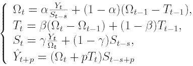
In the middle of last century, Holt proposed an improved method of exponential smoothing, later named after him. In the proposed algorithm, the values of the level and trend are smoothed using exponential smoothing. And smoothing parameters may differ.

Here the first equation describes the overall level of the smoothed series. The second equation is used to assess the trend. The third equation defines the projection of p samples in time forward.
Standing in the smoothing method Holt ideologically play the same role as the constant in the simple exponential smoothing. They are selected, for example, by sorting on these parameters with a certain step. You can use less sophisticated in terms of computational algorithms. The main thing that you can always pick up a pair of parameters, which gives greater accuracy of the model on the test set and then use this pair of parameters in real forecasting.
A special case of the method of Holt is the method of Brown, when a = β.
3.2.3 Method Winters
Although the above-described method of Holt (method of two-parameter exponential smoothing) and is not very simple (with respect to models based on averaging), it does not allow to take into account seasonal variations in forecasting. Speaking more strictly, this method can not make them "see" in the background. There is increased to a three-parametric method is Holt exponential smoothing. This algorithm is called the method of Winters. It attempts to take into account the seasonal components in the data. The system of equations describing the method of Winters as follows:
Fraction in the first equation serves to eliminate the seasonality of Y (t). After excluding seasonal algorithm works with a "clean" data, in which there is no seasonal variations. They appear already in the final prediction, when "pure" forecast, counted almost by the method of Holt is multiplied by a seasonal factor.
3.2.4 Regression methods for forecasting
Along with the above described methods based on exponential smoothing, is long enough to predict the regression algorithms are used. Briefly the essence of this class of algorithms can be described as follows. There is a predicted variable Y (dependent variable) and pre-selected set of variables on which it depends - X1, X2, ..., XN (independent variables).
Model of multiple regression in the general case described by
In a simpler version of the linear regression model, the dependence of the dependent variable from independent has the form:
Here β0, β1, β2, βN matched by the regression coefficients, εcomponent errors. It is assumed that all errors are independent and normally distributed.
To construct the regression models should have a database of observations that looks like this:
| № | X1 | X2 | … | XN | Y |
| 1 | X11 | X12 | … | X1n | Y1 |
| 2 | X21 | X22 | … | X2n | Y2 |
| … | … | … | … | … | … |
| m | Xm1 | Xm2 | … | Xmn | Ym |
Using the table values of past observations, we can choose (for example, the method of least squares) regression coefficients, thereby setting the model.
When working with the regression must comply with some caution and be sure to check on the adequacy of the model found. There are different ways to the test. The essential one is the statistical analysis of residuals, Durbin-Watson test. It is useful, as is the case with neural networks, have an independent set of examples, where you can check the quality of the model.
3.2.5 Methods for Box-Jenkins (ARIMA)
In the mid 90-ies of the last century has been developed fundamentally new and fairly powerful class of algorithms for predicting time series. Most of the work on the study methodology and validation of models was carried out by two statisticians, G.E.P. Boxing (G. E. P. Box) and GM Jenkins (G. M. Jenkins). Since the construction of similar models and obtaining on their basis of forecasts is sometimes called Box-Jenkins methods. For more information hierarchy of algorithms for the Box-Jenkins, we consider below, in the meantime, we note that in this family includes several algorithms, the most known and used of them is the algorithm ARIMA. It is built in almost any special package for forecasting. In the classic form ARIMA not used independent variables. The models are based only on information contained in the prehistory of the projected series, limiting the ability of the algorithm. Currently, the scientific literature often refers to variants of models ARIMA, to take into account the independent variables. Unlike previously discussed methods of forecasting time series in ARIMA methodology is not anticipated any clear model for the prediction of the time series. Set a general class of models describing the time series and allow somehow express the current value of the variable in terms of its previous value. Then the algorithm, adjusting the internal parameters, selects the most appropriate forecasting model. As noted above, there is a whole hierarchy of models of Box-Jenkins. Logically, it can be defined as
AR(p)+MA(q)->ARMA(p,q)->ARMA(p,q)(P,Q)->ARIMA(p,q,r)(P,Q,R)->...
AR (p) autoregressive model of order p.
The model has the form
Y(t)=f_0+f_1*Y(t-1)+f_2*Y(t-2)+...+f_p*Y(t-p)+E(t)
Where: Y (t)-dependent variable at time t. f_0, f_1, f_2, ..., f_p - estimated parameters. E (t) - a mistake from the influence of variables that are not included in this model. The challenge is to determine the f_0, f_1, f_2, ..., f_p. They can evaluate a variety of ways. Correct to search for them via the Yule-Walker equations, for the preparation of this system would require calculation of the autocorrelation function. You can do a simpler way - to calculate their method of least squares.
MA (q)-model with a moving average of order q.
The model has the form:
Y(t)=m+e(t)-w_1*e(t-1)-w_2*e(t-2)-...-w_p*e(t-p)
Where Y (t) the dependent variable at time t. w_0, w_1, w_2, ..., w_p estimated parameters.
3.2.6 Neural network prediction model
Currently, in my opinion, the most promising quantitative method of forecasting is the use of neural networks. We can mention many advantages over other neural network algorithms, here are two basic.
Using neural networks can easily explore the dependence of the predicted value of the independent variables.
Another major advantage of neural networks is that the expert is not held hostage to the choice of mathematical models of behavior of time series. Construction of neural network model is adaptively during training, without the participation of an expert. In this neural network are presented examples from the database and she adapts to the data.
Disadvantage of neural networks is their non-determinism. Refers to the fact that after learning there is a "black box" that somehow works, but the logic of decision-making neural network completely hidden from the expert. In principle, there are algorithms extract knowledge from neural networks ", which formalize the training of the neural network to the list of logical rules, thus creating a network of expert system. Unfortunately, these algorithms are not embedded in the neural network packages to the same set of rules that are generated by such algorithms can be voluminous.
Nevertheless, for people who know how to work with neural networks and knowing the nuances of settings, training and application in practical problems, the opacity of neural networks is not any serious drawback.
The simplest version of the application of artificial neural networks in forecasting problems - the use of conventional perceptron with one, two, or (at most) three hidden layers. In this case the inputs of the neural network is usually served a set of parameters, on the basis of which (the expert's opinion) can be successfully predicted. The solution is usually the weather network in the next time.
Another frequently used neural network architecture used in the prediction of a neural network with general regression. Despite the fact that the principle of learning and application of such networks is fundamentally different from conventional perceptrons external network is used in the same manner as a conventional perceptron. In other words, it is compatible architecture in the sense that a running system, forecasting can be replaced by working on the perceptron network with the overall regression and everything will work. No need to carry out any further manipulation of the data.
Hence the first drawback of such an architecture - when the database is that we expect large network becomes too large and will be slowly working. Since this can be dealt with pre-clustering the database.
4.1 Description of the training and test sample
As a training sample drawn 30 entries from the database MIMIC II Database. These records are divided into 2 groups: group C, which includes records of patients who have not experienced episodes of acute arterial hypotension, and the group H, which includes records of patients experienced an episode of acute arterial hypotension within half an hour after the controlled period.
A test sample consists of ten recordings taken from the database MIMIC II Database. Half of those records - are records of patients who experienced an episode of acute arterial hypotension in half an hour after the control time, while the other half - the recordings of patients who have not experienced episodes of acute arterial hypotension. This sample will be used to control the developed algorithms.
4.2 Program forming time series
In the C programming language using a special API to work with the database MIMIC II Database has developed a program that determines the maximum arterial pressure during the reduction of the left and right ventricles (systole) and minimum pressure during relaxation (diastole). In addition the program determines the duration of these periods of the cardiac cycle.
In this work the formulation of the problem of forecasting episodes of acute arterial hypotension in ICU patients. Forecasting should be based on data available to medical personnel ICU. To develop a system of forecasting as an input is proposed to use a database of physiological signals PhysioNet.
In addition, analysis was carried out scientific and medical literature to examine issues related to blood pressure person. The factors affecting blood pressure. identified the following factors: velichnina cardiac output, minute volume of blood, heart rate, resistance arterioles, the width of the lumen of capillaries and veins, the number and viscosity of blood, vascular tone, humoral system of the organism.
1. The MIMIC II Database http://www.physionet.org/physiobank/database/mimic2db/
2. Chao-Shun Lin, Jainn-Shiun Chiu,Ming-Hui Hsieh, Martin S. Mok, Yu-Chuan Li, Hung-Wen Chiu. Predicting hypotensive episodes during spinal anesthesia with the application of artificial neural networks. Comput. Methods Prog. Biomed. v98 i2. 193-197.
3. Frolich, M.A. and Caton, D., Baseline heart rate may predict hypotension after spinal anesthesia in prehydrated obstetrical patients. Can. J. Anaesth. v49 i2. 185-189.
4. Tarkkila, P. and Isola, J., A regression model for identifying patients at high risk of hypotension, bradycardia and nausea during spinal anesthesia. Acta Anaesthesiol. Scand. V36. 554-558.
5. Subasi, A. and Er?elebi, E., Classification of EEG signals using neural network and logistic regression. Comput. Methods Programs Biomed. V78. 87-99.
6. Hanss, R., Bein, B., Weseloh, H., Bauer, M., Cavus, E., Steinfath, M., Scholz, J. and Tonner, P.H., Heart rate variability predicts severe hypotension after spinal anesthesia. Anesthesiology. v104. 537-545.
7. Textbook of Physiology (Bykov, Vladimirov, Business, Conradi, Slonim). Medgiz 1955;
8. Pathological Physiology (A.D. Ado, M.A. Ado);
9. Ophthalmologic symptoms in congenital and acquired diseases (M.D. Agatova).
10. Human Anatomy. S. Mikhailov, LL Kolesnikov, VS Bratakov. 3rd ed., Rev. and expanded. - M.: Medicine, 1999 - 735s.
11. Human Anatomy. In 2 vols. V.2. EI Borzyak, VY Bocharov, MR Sapin et al, Ed. MR SAPINA. - 2 ed. rev. and add. - M.: Medicine, 1993 - 560p.
12. V.I. Maksimov. Fundamentals of anatomy and physiology. M.: KolosS, 2004 - 167s.