Field simulation for RFID-based in door location sensing algorithm
Sebastian Rubin
Источник: http://www.cse.ust.hk/~zgu/comp680g/projects/RubinWSN.pdf
Abstract
In recent years, positioning systems for indoor areas using the Radio Frequency Identification (RFID) infrastructure have been suggested. Such systems make use of location fingerprinting algorithm for determining the location of object carrying RF tag. However, due to the environmental influence, theoretical model for these algorithms often fails to function in real world application, which necessitates sufficiently testing of any proposed system. Our project aims at providing a simulator which leverages Ptolemy environment to support high-fidelity simulation of RF system. By this simulator, developers can evaluate their locating algorithm before expensive road-test. The hypothetic RF signal propagation model is introduced. And a sample algorithm, LADDMARC, is implemented to evaluate our simulator.
1 Introduction
Recently there is a new approach to the in-door location sensing problem [8], which is build on top of the Radio Frequency Identification (RFID) technology. In this solution, several equipments, particularly the RFID reader and RF tag, are used to gather signal data sets. The signal data sets which have been acquired by the RFID readers then serve as arguments for localization algorithms such as triangulation [2]. In the real world, researchers in this emerging field come across many problems. A most serious one among them is the environmental influence. Due to the characteristic of the equipment, RFID applications severely suffer from environmental influence. This may even break the theoretical assumptions made in the location sensing models and cause them to fail in real applications [1]. Thus, it is very important for practical algorithms to take environmental influence into consideration. However, because the pattern of potential environmental influence is difficult to fully observed, algorithm adaptation according to environmental factors can not be justified formally. On the other hand, due to some limitations which we will be discussed in more detail in section 3, the road-test evaluation of RFID-based location sensing system is very costly. Thus, the thorough evaluation of their precision, performance, scalability and stability is very difficult.
Facing this problem which hinders the researches on RFID location sensing, our project aims at providing a high-fidelity simulation program in which both the behavior of RFID equipment and the influence exerted by the environment are simulated. Using the proposed program, a developer can easily gather the statistic data by simulating his algorithm in different configurations resulting in a cost which is relatively low. The simulation result facilitates preliminary analysis of precision, performance, scalability and stability of each algorithm. It can also be used as an indicator to help researchers determine whether expensive road-tests on certain configurations should be carried out.
In order to leverage existing simulation technique. We build our simulator on top of Ptolemy framework [7]. Ptolemy is an ongoing project at UC Berkeley that studies modeling, discrete-event simulation, and design of concurrent, real-time, embedded systems. The key underlying principle in Ptolemy is the ability to use multiple models of computation in a hierarchical heterogeneous design environment, which is of particular importance to RF system simulation, since for the wireless channel and relevant devices there need different simulation models.
The remaining part of this report is organized as follows: Section 2 briefly introduces the RFID technology and RFID-based indoor location sensing algorithm. Section 3 describes several practical problems encountered in the above mentioned research. Next, section 4 has an overview of our project, including the objectives and the architecture. Then section 5 describes how to model and simulate in Ptolemy. Section 6 describes the signal propagation model. Section 7 reports our implementation. And at last section 8 evaluates our work by introducing LANDMARC simulation.
2 Background
2.1 Location sensing
Pervasive computing is a convergence of many techniques such as embedded systems and mobile computing. Nowadays it becomes more and more important and is regarded as the next generation of computing paradigm. In pervasive computing, a most important issue is context management. Contexts can model many factors in pervasive computing. For example, temperature, velocity, signal strength can all be considered to be a kind of context.
For many context-aware applications, location is an essential part of context. For example, in a large-scale warehouse, a goods tracing system may be deployed to continuously monitor the location of the goods. This location information is then utilized later to guide the deliverer to approach the desired goods. Due to the importance of location context, a lot of research work has been conducted to find efficient location sensing algorithms in different configurations. These configurations involve various types or settings of signal transportation media and infrastructure, and thus meet different requirements. For example, the Global Positioning System (GPS) deploys 24 satellites around the orbit and utilizes long wave radio signal to perform the locating. It is a particular solution for out-door location sensing. However, for in-door location sensing, GPS is unsuitable.
2.2 RFID technology
RFID is a technology to store and retrieve data through electromagnetic transmission to an RF compatible integrated circuit. A RFID system consists of two basic components, the RFID reader and the RF tag, as illustrated in figure 1. The RFID reader can read data emitted from RFID tags through a predefined radio frequency and protocol to transmit and receive data. Basically there are two kinds of RF tags: the passive tag and active tag. Passive tags operate without battery. They can not emit RF signal on their own. The basic function of them is to reflect the signal transmitted by the RFID reader while modulating the reflected signal to add burned-in tag information. By contrast, active tags carry on-board radio transceivers and batteries. With continuous RF signal emission enabled by power supply, they are capable of actively communicating with the RFID reader.
Passive RFID tag is mostly used as a replacement of traditional bar-code technology. Although they have many advantages such as unlimited operating

Figure 1: RFID reader and RF tag
lifetime, lower cost and less weight, they also have a severe drawback that make them unsuitable for location sensing: the limited sensing range. On the other hand, the active tags have a much longer sensing range (typically 0-50m [9]) and their omitted signal follow a measurable power propagation pattern (a reasonable hypothesis is that the signal strength will drop continuously as the distance between the tag and the receiver increase). These factors make active tag almost the only choice for RFID-location sensing applications.
2.3 RFID-based indoor location sensing
Originally, the RFID technique was proposed mainly for object identification. For object identification, the location context is of little use. However, since the field or wave delivered from an antenna extends into the space surrounding the RFID reader and its strength diminishes with respect to distance, object tracing by RF signal is also possible. An example of the RFID-based location sensing algorithm is the the LANDMARC algorithm [8].
2.4 The LANDMARC algorithm
In order to increase accuracy without placing more readers, the LANDMARC (Location Identification based on Dynamic Active RFID Calibration) system employs the idea of having extra fixed location reference tags to help location calibration. These reference tags serve as reference points in the system (like landmarks in our daily life). As figure 2 illustrates, in the LANDMARC algorithm both reference tags and tracing tags are active RF tags. Each reference tag is placed in one grip node, and the tracing tag may move freely inside the grip. And all four deployed RFID readers can output pairs of signal strength and tag identification. The location of the reference tags are known in advance, and thus the algorithm can figure out the location of the tracing tag by comparing its signal strength with those of the reference tags.

Figure 2: LANDMARC algorithm
The proposed approach has three major advantages over preliminary solutions that did not use reference tags. First, there is no need for a large number of expensive RFID readers. Instead extra, cheaper RFID tags are used. Second, the environmental dynamics can easily be accommodated. The LAND-MARC approach helps offset many environmental factors that contribute to the variations in detected range because the reference tags are subject to the same effect in the environment as the tags to be located. Thus, the reference information can dynamically be updated for lookup based on the detected range from the reference tags in real-time. Third, the location information is more accurate and reliable. The LANDMARC approach is more flexible and dynamic and can achieve much more accurate and close to real-time location sensing.
3 Problems
According to a research conducted to investigate the LANDMARC’s precision [1], it is found that this algorithm behaves poorly in a particular laboratory environment. In this experiment, a tracing tag is moved across a distance of 1 to 3 meter, but the location change calculated from LANDMARC is only within 0.2 meter. This fact indicates the importance of carefully and thoroughly evaluating theoretical models and algorithms on different configurations.
However, evaluating RFID location sensing algorithms on different configurations by road-tests is by no means an easy task due to some realistic problems listed below:
1. Experimental field restriction: Due to space limitations of the laboratory, the experimental field usually has a limited size and a fixed shape. For example, the research conducted in [1] is carried out in a room with maximum square size of about 7*7 meter. However, even if the algorithm behaved well in this area (actually it does not), whether it guarantees the same accuracy in a larger area is in doubt.
2. Equipment availability: Currently a typical RFID-reader costs more than $10000, excluding the auxiliary appliances. The price of a typical RFID tag is relatively cheap. However, the amount of RFID tags need to be used may be very high. Thus the total cost may well exceed the budget of the researchers who want to evaluate the scalability of their algorithm. Besides, different readers and tags may have different characteristics, which make thing worse.
3. Test duration limitation: The stability issue is another concern. Algorithms may behave well for a short period of time, but ill-behave afterward. According to the above mentioned inves-
tigation [1], this phenomenon does exist. Whatever the reason is, it justifies the need for continuously testing the algorithm for a long period of time. For road-tests, this may be very costly.
To overcome this problems, we suggest the simulation approach. The next section provides an overview of the simulation program.
4 Overview of the RF simulator
The main objective of our project is to enable evaluation of different RFID-based location sensing algorithm’s precision, scalability and stability in the simulation environment. This simulation environment is provided as a easy-to-use application for the researchers.
Figure 3: General architecture for simulation program
For this simulation program, we have identified the following five key capabilities:

• Equipments simulation: The program must be capable of simulating the characteristics of different equipments. Basically we need to consider four essential equipments: the RFID-reader, the active RF tag, the data collector and the controller. The RFID-reader and RF tag have already been introduced above. The data collector simulates a real-world equipment which gathers signal strength data sent by readers. On the other hand, the controller simulates an equipment which may change the setting of readers upon certain triggers. Typically both the data collector and the controller are all programs running on a PC which communicates with the RFID readers by ethernet or 802.11 protocol.
• Calibration: Simulating the environmental factors is one of the main motivations of our project. These factors exert their influence on the precision of the algorithm by disturbing the relation between signal strength and the distance. For example, figure 4 referred to from [1] shows that due to environmental factors, the relation is far from monotony which is assumed by the LANDMARK algorithm. This indicates that the RF signal is sensitive to environmental factors. Currently our project encode a calibration sub-system to encode these enviromental factors.
• Algorithm interface library: Since the main target is to perform evaluation on different location sensing algorithms, it is very important to provide an interface library for the researchers to implement their algorithm into the simulation program. This interface library defines a set of components as well as their functional specifications, and should also be well documented. The researchers will develop algorithm plugins
on top of this interface library.
• Simulation engine: The simulation is based on a discrete-time model. Each run can last for a certain period of time. The simulated tracing RF tag may stay at the same place or it may move along a special path with a pre-set speed. The simulated RFID readers will generate signal strength data at certain time interval and send them to the data collector. The data collector in turn labels the data and sends them to the location-sensing algorithm for further evaluation. This whole process is simulated in the engine.
• Visualization: The visualization includes two parts. The first part is a graph-based editor which allows the user to define the experiment configuration by simple drag-and-drop of equipment and environment components. Besides, the properties of these components can be set in user-friendly dialogs clearly explaining the usage. The second part is to visualize the simulation results in different kinds of plots, which facilitates further analysis.
According to these objectives, we design an architecture for our simulation program, as figure 3 illustrates. Each component copes with certain capabilities.
5 Modeling and simulating with Ptolemy II
To achieve the above mentioned objectives we alleviate the workload by reusing existing simulation techniques. In order to reuse existing simulation techniques as much as possible, we cultivate the Ptolemy II simulation system and decided to build our RFID simulation system on top of it. In this section, we
introduce the Ptolemy II simulation system for embedded systems, the VisualSense visual editor and simulator for wireless sensor network systems and then propose the basic idea of how to build our simulation program.
5.1 Ptolemy II
Ptolemy [7] is an ongoing project at UC Berkeley that studies modeling, discrete-event simulation, and design of concurrent, real-time, embedded systems. The key underlying principle in Ptolemy is the ability to use multiple models of computation (e.g., continuous-time, dataflow, finite-state machines) in a hierarchical heterogeneous design environment. Ptolemy II is a software framework developed as part of the Ptolemy project. It is a Java-based component assembly framework with a graphical user interface called Vergil and a step further in the development of the classic Ptolemy which was written in C++ and had a far simpler graphical user interface. Major reasons for developing Ptolemy II as an advancement of the classic Ptolemy were to exploit the network integration, migrating code, built-in threading, and user-interface capabilities of Java. Ptolemy II introduces the notion of domain polymorphisms where components can be designed to be able to operate in multiple domains and modal models where finite state machines are combined hierarchically with other models of computation. Ptolemy II also contains a continuous-time domain, which combined with the modal modeling capability, yields hybrid system modeling. Ptolemy II furthermore has a sophisticated type system with type inference and data polymorphisms where components can be designed to operate on multiple data types, and a rich expression language. The concept of behavioral types emerged where components and domains could have interface definitions that describe not just static structure, as with traditional type systems, but
also dynamic behavior.
As for code generation, the tactic in Ptolemy II is significantly different than that in Gabriel, or Ptolemy Classic, with Gabriel being the predecessor of Ptolemy Classic. Instead of components as generators, Ptolemy II uses a component specialization framework built on top of a Java compiler toolkit called Soot. Ptolemy II uses XML for its persistent data representation, and has introduced the concept of migrating models.
5.2 VisualSense
VisualSense is a modeling and simulation framework for wireless and sensor networks that builds on and leverages Ptolemy II. Modeling of wireless networks requires sophisticated representation and analysis of communication channels, sensors, ad-hoc networking protocols, localization strategies, media access control protocols, energy consumption in sensor nodes, etc. This modeling framework is designed to support a component-based construction of such models. It supports actor-oriented definition of network nodes, wireless communication channels, physical media such as acoustic channels, and wired subsystems. The software architecture of Vi-sualSense consists of a set of base classes for defining channels and sensor nodes, a library of subclasses that provide certain specific channel models and node models, and an extensible visualization framework. Custom nodes can be defined by subclassing the base classes and defining the behavior in Java or by creating composite models using any of several Ptolemy II modeling environments. Custom channels can be defined by subclassing the Wireless-Channel base class and by attaching functionality defined in Ptolemy II models. Thus, it provides a component-based framework to build the simulation program, which can be used as the basis our work.
6 RF Signal propagation model
Let us first clarify the problem setting. Consider an RF indoor positioning system overlaid on a single floor. We assume that there are N RF readers in the area and they are all visible throughout the area under consideration. A square grid is defined over the two dimensional floor plan and any estimate of RF tag location is limited to the points on this grid. Assuming that the grid spacing results in L points along both the x and y axes. we have L × L positions in the area. Any position can be represented by a triplet with label (x, y) where x and y represents the 2-D coordinates on the floor plane.
For this problem setting, we have performed an experiment to find the relation between signal strength and distance from reader to tag, as figure 4 shows. Here we can see that the relation is roughly a logarithmic function. However, the environmental influence is very strong, and the signal strength actually can not be uniquely estimated by distance. Figure 5 and 6 shows the signal strength distribution collected by 4 readers along a 10 × 10 grip. Because currently we still can not find how to model the environmental influence, we decide not to use the logarithmic function directly. Instead, we use the calibration data to estimate the signal strength. This approach is justified by research [3].
The calibration records are collected for the predetermined points on the grid with enough statistics (we explain this below). A total of K entries are recorded in the database. If the signal strengths are measured at each point on the grid. Then K = L2. Occasionally. some points on the grid are not accessible for measurement and are left out of the database. Each entry in the calibration database includes a mapping of the grid coordinate (x, y) to the vector of corresponding signal strength values from all

Figure 5: Signal Strength Distribution for 10*10 grip, Reader 1 and Reader 2

Figure 6: Signal Strength Distribution for 10*10 grip, Reader 3 and Reader 4
RF readers in the area. Note that the received signal strength is recommended by [4] because it exhibits a stronger correlation with location than the signal-to-noise ratio (SNR).
Note that the finding in [4] indicates that the signal strength of the same location varies depending on the user’s orientation. Currently the calibration records are achieved by collecting a large number of samples of the signal strength for each orientation of the tag and the reader antenna. Thus we assumes that the variations due to orientation have been averaged out when the signal strength is recorded for all positions.
The rationale for assuming that the signal strength is a normally distributed random variable is as follows. Measurements of the signal strength in many locations over the last few decades seem to support the fact that RF signal is lognormally distributed [5]. Some measurement results [6] support this assumption as well. The measurement of the signal strength in an office room over long time periods ranging from five hours, 20 hours and one month showed that it had a standard deviation a of 2.13. Small et. al. also reported that signal did not vary dramatically at different times of the day. At the same time, some of our own measurements over smaller durations of time indicate that this assumption may be valid only in certain situations. However, we use this distribution in this preliminary model for mathematical tractability. The assumption of independence is acceptable since there is no relationship between the signals transmitted by different RF readers.
Now according to this model, we estimate the sig-
Figure 4: Relation between RFID signal strength and distance with heavy environmental influence
Now two vectors are used in estimating the signal strength at given position. The first vector consists of samples of the RF signal strength measured at the RF signal readers from N access points in the area. We call it the sample vector. This vector is denoted as: S = [p\, p2, ■■■pn]. Each component in this vector is assumed to be a random variable with the following assumptions:
• The random variables pi for all i are mutually independent
• The random variables pi are normally (or Gaussian) distributed
• The (sample) standard deviation of all the random variables pi is assumed to be identical and denoted as a
• The true mean of the random variable pi is denoted as Ti, which can be retrieved from the calibration record.
The second vector. that forms the fingerprint of the location, consists of the true means of all the received signal strength random variables at given location

nal strength for location (x,y) in this way:
1. First find M nearest neighbors to location (x,y) in calibration database as R\, R2, R%...Rm. M is a parameter for this model, normally we take 4 as its value.
2. Next for each neighboring vector Ri = [r\, Г2, ■■■тп], we perform n random processes to determine the estimated signal Si = [pi, P2, ■■■Pn] by the following formula. Note that a as standard derivation is another parameter for the model, according to [6], we take a value of 2.13.
3. Once we have S\, S2, Ss...Sm we perform an average to get the estimating signal strength for the given location.
7 Implementation of RF Simulator
In this section, we first introduce how to use our program to perform RFID simulation, then discuss the implementation details.
7.1 Running the program
The most important components and their basic functions are listed as follows and their implementation details are discussed in section 7.2.
• RFWirelessDirector: As a director, RFWire-lessDirector governs the execution of a RF simulation model. When the model is started, it calls the fire method of the top-level component. By contrast to other directors such as DEDirector, RFWirelessDirector has 2 execution modes: Calibration mode and Simulation mode.
• RFGrip: An auxiliary component to help developers to map the geometry distance from the real world experiment field to the simulation model. There are three arguments for this component: column grip count, row grip count and grip size in real world units.
• RFWirelessChannel: Used in both simulation mode and calibration mode. Implements the RF Signal propagation model. All signal-involved components in a RF simulation model should set their channel name to be the same existing RFWirelessChannel in order to get the signal input or output. To use this class, place it in an RFID simulation model that contains a RFWirelessDirector and other RFID actors that contain port instances of WirelessIOPort. Then set the outsideChannel parameter of those ports to match the name of this channel. The model can also itself contain ports that are instances of WirelessIOPort, in which case their insideChannel parameter should contain the name of this channel if they should use this channel. Transmission of RF signal on a channel reaches all ports at the same level of the hierarchy that are instances of WirelessIOPort and that specify that they use this channel. These ports include those contained by entities that have the container as this channel and that have their outsideChannel parameter set to the name of this channel. They also include those ports whose containers are the same as the container of this channel and whose insideChannel parameter matches this channel name.
• CalibrationTag: Used in calibration mode. Communicate with the RFWirelessChannel RF reader device driver to get the real world RF signal. It is the responsibility of the developer to

place the real calibration tag to the correct location. Otherwise the calibration may fail.
• RFCalibrationFile: Written in calibration mode, read in simulation mode. Each calibration file contains several rows, each row records a 2D location and corresponding signal strength for all readers.
• RFTag: Used in simulation mode, for every 2 seconds transmitted signal out of the RFWire-lessChannel. The content of the signal includes the tag ID.
• RFSignalReader: Used in simulation mode. This component has a WirelessIOPort as input port and a normal IO Port as output port. Via the input port it receives the signal token as transmitted by the RFTag through the RFWireless-Channel. The output port is linked to the implementation of the locating algorithm and it outputs the signal strength, tag ID and reader ID to locating component, such as the LANDMARC locater.
Now we go through the simulation process step by step. As previously stated, the environmental factor is encoded in the calibration records. Thus, the first step of any simulation is to calibrate the signal propagation model. To this step, we have to write several components. Besides, for the director, there is a special mode called calibration mode.
The calibration setting is illustrated in figure 7. In the sample setting we use a 10 × 10 grip. Four readers are placed at each corner. The “mode” property of RFWirelessDirector is set to be “Calibration” and “directory” property which specify file location of calibration file is also set.

Figure 7: Calibration Setting
While performing calibration, we put the calibration tag at each position and then click the “start” button in Ptolemy. Then four windows pop up to record the progress of calibration, as figure 8 illustrated. We wait until signal strength for all readers are stable. Then click the “stop” button. Then those signal strengths are recorded in the calibration file. From the calibration records we know the true means of each grip location.
After calibrating the model, the algorithm can be simulated. Here figure 9 illustrates a basic simulation setting. A more complicated example is discussed in section 8. In figure 9, an RF tag is placed inside the grip and every 2 second it outputs an RF signal. Four readers receive the signal token through RFWireless-Channel, and output the signal strength, tag ID and reader ID onto a display.
7.2 Implementation detail
As previously mentioned, the RFWirelessDirector governs the execution of a RF simulation model. More precisely, ptolemy defines the director of an actor to be either its local director (if it has one) or its executive director (if it does not). A local director is responsible for execution of the components within the composite. It will perform any scheduling that might be necessary, dispatch threads that need to be started, generate code that needs to be generated, etc. On the other hand, inside the composite components there is a executive director associated with an actor that is responsible for firing the actor. A composite actor that is not at the top level has as its executive director the director of the container. Every executable actor has a director except the top-level composite actor, and that director is what is returned by the getDirector() method of the Actor interface. A composite actor that is not at the top level may or may not have its own local director. The RFWire-lessDirector acts as a local director for the top-level component in the RF simulation model.
The class diagram and general execution sequence is illustrated in figure 10 and 12. When any action method is called on an opaque composite actor, the composite actor will generally call the corresponding method in its local director. This interaction is crucial. Here we briefly discuss the overall process. When a director is initialized, via its ini-tialize() method, it invokes initialize() on all the actors in the next level of the hierarchy, in the order in which these actors were created. The wrapup() method works in a similar way, deeply traversing the hierarchy. In other words, calling initialize() on a composite actor is guaranteed to initialize in all the objects contained within that actor. Similarly for wrapup(). The fire() method is where the bulk of work for a director occurs. When fire() is called in the director, the fire() method of the director invokes

Figure 8: Observe the calibration progress

Figure 9: Basic simulation setting

Figure 10: Class diagram of Ptolemy framework
the prefire() method of all the actors before invoking any of their fire() methods. Then the fire() method of the director selects an actor that return true for the prefire() method, invokes its fire() method some number of times followed by its postfire() method.
The class hierarchy for components is shown in figure 11. Here we introduce the implementation details for each important class.
Class RFWirelessDirector implements the director. It has a boolean property as a switch to select between calibration mode and simulation mode. In the fire method, the RFWirelessDirector acts according to current mode. In calibration mode, only RF-

Figure 11: Class diagram for main component in the simulation program
CalibrationTag and RF reader is fired. RFCalibra-tionTag uses RFDeviceReader to receive device sig-1n.1,a <ldeafanultd> transmit to reader to record. Only one RF-CalibrationTag is allowed in any mode in calibration mode, otherwise an exception is throwed. On the other hand, in simulation mode RFCalibrationTag is omitted. The RFWirelessDirector querys each components by their prefire() method and then fire those that return true.
Class RFWirelessChannel implements the RF signal channel. In the fire() method, this class reads the input signal token transmitted by the RFTag or RFCalibrationTag, and then use the location of the source tag to determine signal strength for each reader(the location of source tag can be easily retrieved by visiting the “ location” property). The model described in section 6 and calibration data are applied to serve this purpose. In the output signal, the tag ID is also included.
Class RFTag component implements the tag for

Figure 12: Sequence diagram of Ptolemy framework
simulation. Actually this component is not implemented by a java class. Instead, it is implemented by a composite actor. In this actor a DEDirector is deployed to act as local director. And a timed source, clock, stimulates a output port every 2 seconds. The output port is linked to RFWirelessChannel in top-level model and output a string parameter of this composite actor as tag ID.
The RFDeviceReader encapsulates the communication with the device driver for the RF reader. Currently only one kind of device, Mantis II from RF Code corporation, is supported. The communication is through TCP socket.
Class RFSignalReader implements the reader for simulation. This component has a WirelessIOPort as input port and a normal IO Port as output port. In the fire() method, it retrieves the signal token transmitted by RFTag through RFWirelessChannel. The token includes signal strength and Tag ID for the source tag. Then it adds the reader ID into the record and
outputs this record through the output port.
8 Evaluation
We implement the LANDMARK algorithm to evaluate our simulator program. The experiment setting is illustrated in figure 13 and figure 14. In figure 13,

Figure 13: Simulating Tag by Composition Actor

Figure 14: Running the simulation for LANDMARC algorithm
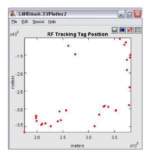
Figure 15: LANDMARC simulation result
we model a RF tracking tag that transmit an RF signal every 2 second while moving one step around a circle every 3 second. This composite actor is driven by a DEDirector.
In figure 14, we demonstrate a typical LAND-MARC locating application. There are 10 ∗ 10 grips with 4 readers at each conner. for each grip there is a reference tag whose location is known in advance. Besides, a special component, the LANDMARCLo-cator, is provided to simulate LANDMARC algorithm on the signal strength of both tracking tag and reference tag. The output of LANDMARCLocator is an array encoding estimated location.
Finally, the simulation result is shown in figure 15.
References
[1] X. Chang. Towards improved data quality for RFID applications. Group meeting, Sep 2005.
[2] J. Hightower and G. Borriello. Cse 01-08-03: A survey and taxonomy of location sensing systems for ubiquitous computing. Technical report, University of Washington, Department of Computer Science and Engineering, Aug 2001.
[3] K. Kaemarungsi and P. Kristhnamurthy. Modeling of indoor positioning system based on location fingerprinting, March 2004.
[4] P.Bahl and V. Padmanabhan. Radar: An in-building rf-based user location and tracking system, 2000.
[5] T. Rappaport. Wireless communications: Principle and Practice. Prentice Hall PTR, Upper Saddle River, New Jersey, 1996.
[6] J. S. A. Smailagic. and D.P.Siewiorek. Determining user location for context aware computing through the use of a wireless lan infrastructure. Technical report, CMU, Dec 2000.
[7] Jie Liu and E. A. Lee. A component-based approach to modeling and simulating mixed-signal and hybrid systems. ACM transactions on Modeling and Computer Simulation(TOMACS), 12(4), October 2002.
[8] Lionel M, Yunhao Liu, Yiu Cho Lau, and A. P. Patil. LANDMARC: Indoor location sensing using active RFID. Wireless Networks, 10(6), Sep 2005.
[9] RF Code, Inc. http://rfcode.com/productsframe.asp.