ON THE MODELING AND ANALYSYS OF JITTER IN ATE USING MATLAB
Kyung Ki Kim, Jing Huang, Yong-Bin Kim, Fabrizio Lombardi
Čńňî÷íčę:
www.ece.neu.edu/groups/hpvlsi/publication/On_MODELING_ANAYLYSYS
Abstract
This paper presents a new jitter component analysis method for mixed mode VLSI
chip testing in Automatic Test Equipment (ATE). The separate components are
analyzed individually and then combined using Matlab. The Matlab simulation
shows how jitter components combine and how the total jitter depends on the
jitter injection sequence. The relationship among jitter components is presented
and the superposition of the jitter components is verified. This new technique
gives test engineers an insight into how the jitter components interact.
1. Introduction
As the data rates of VLSI systems reach several gigabits per second, timing
jitter have become more significant in ATE (Automatic Test Equipment) systems.
Therefore, a correct model and analysis of the timing errors and jitter will
provide more accurate characterizations of high-speed VLSI systems. Timing
Jitter (henceforth referred to as jitter) is defined as the deviation of a
signal transition from its ideal position in time. The Total Jitter (TJ)
consists of two components: the Deterministic Jitter (DJ) and Random Jitter
(RJ). Assuming that the each jitter component is independent, the distribution
of TJ will be the convolution of the distributions of DJ and RJ. The DJ consists
of several subcomponents. These may include Electromagnetic Interference,
Cross-Talk, Bandwidth Limitation, and etc. DJ has a bounded peak-to-peak value
that does not increase when more samples are taken.
The RJ comes from device noise sources such as thermal and flicker noise. It is
theoretically unbounded in amplitude, and is characterized by a Gaussian
distribution. Multiple random jitter sources add in an rms fashion, but a
peak-to-peak value is needed to get total peak-to-peak jitter when RJ is
combined with DJ. Although Gaussian statistics imply an "infinite" peak-to-peak
amplitude, a useful peak-to-peak
value can be calculated from the rms value after a probability of exceeding the
peak-topeak value is established. For example, the peak-to-peak random jitter
has less than 10-12 probability of exceeding is 14.1 times the rms value [1].
Many works have been reported on jitter measurement and analysis. It is
relatively simple to measure each jitter component but it is challenging to
measure and analyze them if multiple jitter components are simultaneously
injected. However, there has not been a consensus on a standard methodology for
separating measured total jitter into components. Only a few methods such as the
Tailfit Algorithm, One-Shot Time Interval Methodology, and Spectral Methodology
have been proposed on the this critical issue [2][3][4][5].
The objective of this paper is to determine how jitter components can be modeled
and combined, and how the total jitter can be changed according to different
injection sequence. In this paper, a novel and standard amenable jitter
component analysis and combining methodology are proposed, and Matlab is used to
demonstrate the effectiveness of the methodology. The remainder of this paper is
organized as follows. Section 2 shows the jitter classification and the
definition of each model for the components. Section 3 presents jitter combining
and measurement experiments followed by conclusion in Section 4.
2. Jitter Classification
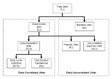
Deterministic Jitter (DJ) consists of Duty-Cycle Distortion (DCD), Inter-Symbol
Interference (ISI), Periodic Jitter (PJ), and Bounded Uncorrelated Jitter (BUJ).
DCD and ISI are referred to as data correlated jitter, while PJ, RJ and BUJ are
referred to as data uncorrelated jitter [6][7]. Figure 1 shows a block diagram
of the jitter classification. Accurate jitter models and their analysis are
essential for better prediction and characterization of jitter effects in
high-speed VLSI systems.
Figure 1. Jitter classification
2.1. Periodic Jitter (PJ) Model
Electromagnetic Interference (EMI) can cause a periodic deviation of a signal
transition from its expected location. This type of deviation is referred to as
Sinusoidal or Periodic Jitter, which repeats in a cyclic fashion. PJ is
typically uncorrelated to any periodically repeating patterns in the data
stream. The model of PJ is summation of cosine functions with phase deviation,
modulation frequency, and peak amplitude [6]. The model is represented by

where PJTotal(t) denotes the total periodic jitter, N is the number of cosine components (tones), Ai is the amplitude in units of time, ωi is the modulation frequency, t is the time, and θi is the initial phase.
2.2. Duty Cycle Distortion (DCD) Model DCD results in high bit cells having a different width from low bit cells. It is caused by a difference in propagation delay between low to high transitions and high to low transitions. The sources of the DCD can be offset errors, turn-on delays and saturation. Figure 2 is the proposed DCD model that generates the duty cycle effect in a signal.

Figure 2. DCD model
2.3. Inter-Symbolic Interference (ISI) Model ISI is dependent on the data pattern, date rate, data slew rate, and frequency response of the data path. The step response of ISI model might be approximated by the threepole response. Therefore, our ISI model is a 3-pole LPF system that consists of a 1-pole and 2-poles LPF system. It is given by
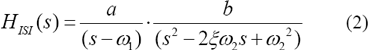
where a and b are constants. ω1 is a
single pole of the 1-pole system; ω2 is the natural frequency and ξ is the
damping ratio of the 2-poles system. The ISI model may not reflect all the
effect of a lossy line, which is the dominant cause of ISI in the real world,
but if the settling time of the 3-pole LPF system is greater than 2-bit Unit
Interval (UI), it will be a good estimate to the lossy line [8].
High-frequency losses caused by the skin effect and dielectric loss also affect
ISI. These effects are frequency-related. The skin effect is proportional to the
square root of the frequency, while the dielectric loss is proportional to the
frequency [9]. Therefore, the skin effect dominates data loss at a lower
frequency, whereas the dielectric loss dominates at a higher frequency.
2.4. Random Jitter (RJ) Model
RJ is theoretically unbounded in amplitude, and is characterized by both Gaussian and non-Gaussian Distributions. In this paper, it is assumed that RJ has simple Random Gaussian distribution (like thermal and flicker noise) and it is given by

where σ is the standard deviation of
the jitter distribution or the rms value, and JRJ is the probability that the
edge will occur at time x, where x is the deviation from the mean value of the
transition time.
The observed effect of RJ depends on the number of samples. The relationship
between rms and peak-to-peak jitter conversion as shown in Equation (4) is used
to compute the peak-to-peak jitter [1]. This relationship is given by

Conclusion
This paper has developed models of jitter components and jitter combining
methods using Matlab as a simulator of an ATE system. In the jitter modeling, PJ
model was a single-tone sinusoidal jitter, RJ was a Gaussian noise signal, ISI
model was a 3-pole LPF, and DCD model generated the duty cycle effect of a
signal. The components models have been developed and characterized in order to
predict overall system jitter.
It has been demonstrated how jitters combine, and how the jitter varies with
jitter injection sequence. Matlab was used to inject each subcomponent in five
injection sequences. The jitter rms values and peak-to-peak values were compared
with one another. The convolution of each jitter components was presented, and
compared with the TJ of each jitter combining. As a result, it has been shown
that TJ does not depend on the jitter injection sequence, and that superposition
applied. The jitter modeling and combining method using Matlab should contribute
to standardization of a total jitter simulation. More detailed models are
currently under development.
References
[1] Maxim, “Converting between RMS and Peak-to-Peak Jitter at a Specified BER.”
Application Note, HFAN- 4.0.2, Rev1; 2/-3;
http://pdfserv.maxim-ic.com/arpdf/AppNotes/3hfan402.pdf
[2] Mike P.Li, Jan Wilstrup, et. al, “A New Method for Jitter Decomposition
Through Its Distribution Tail Fitting.” IEEE International Test Conference,
pp788-794, 1999
[3] Jan Wilstrup, Corporate Consultant, “ A Method of Serial Data Jitter
Analysis Using One-Shot Time Interval Measurements.”, IEEE International Test
Conference, page 819-823, Oct. 1998.
[4] John Patrin, Mike Li, “Comparison and Correlation of Signal Integrity
Measurement Techniques,” DesignCon 2002.