Predictive Models for Proactive Network Management: Application to a Production Web Server
Ссылка на оригинал.Dongxu Shen Joseph L. Hellerstein
Rensselaer Polytechnique Institute IBM T. J. Watson Research Center
Troy, NY 12180 Hawthorne, NY 10598
shend@rpi.edu hellers@us.ibm.com
Proactive management holds the promise of taking corrective actions in advance of service disruptions. Achieving this goal requires predictive models so that potential problems can be anticipated. Our approach builds on previous research in which HTTP operations per second are studied in a web server. As in this prior work, we model HTTP operations as two subprocesses, a (deterministic) trend subprocess and a (random but stationary) residual subprocess.
Herein, the trend model is enhanced by using a low-pass filter. Further, we employ techniques that reduce the required data history, thereby reducing the impact of changes in the trend process. As in the prior work, an autore-gressive model is used for the residual process. We study the limits of the autoregressive model in the prediction of network traffic. Then we demonstrate that long-range dependencies remain in the residual process even after autore-gressive components are removed, which impacts our ability to predict future observations. Last, we analyze the validity of assumptions employed, especially the normality assumption.
Network traffic prediction, traffic modeling, AR model, network management, web server.
Network robustness is a central concern for information service providers. Network failures will, at a minimum, cause user inconvenience. Often, failures have
a substantial financial impact, such as loss of business opportunities and customer dissatisfaction. Forecasting service level violations offers the opportunity to take corrective actions in advance of service disruptions. For example, predicting excessive web traffic may prompt network managers to limit access to low priority web sites.
Forecasting is common in areas as diverse as weather prediction [2] and projections of future economic performance [3]. However, not enough has been done on network traffic. Herein, we address this area. However, due to the burstiness and non-stationarities of network traffic, there are inherent limits to the accuracy of predictions.
Despite these difficulties, we are strongly motivated to develop predictive models of networked systems, since having such models will enable a new generation of proactive management technologies. There has been considerable works in the area of fault detection [6, 7]. There are some efforts in proactive detection[5, 8].
Our work can be viewed as a sequel to [8]. This paper studies the number of hypertext protocol (HTTP) operations per second. The data are detrended using a model of daily traffic patterns that consider time-of-day, day-of-week, and month, and an autoregressive model is used to characterize the residual process. Here we use the same dataset and variable. Also, as in the prior work, we employ separate models of the non-stationary (trend) and stationary components of the original process. However, we go beyond [8] in the following ways:
1. We provide a different way to model the trend so that less historical data are needed.
2. In obtaining the trend model, we use a low pass filter to extract more structure from the data.
3. The assumptions underlying the residual process are examined in more details, especially the assumption of a Gaussian distribution.
4. Both the current and prior work use autoregressive (AR) models for forecasting. In the current work, we shed light on the limits of AR-based predictions.
5. We show that long-range dependencies remain in the data even after the trend and is removed. This situation poses challenges for prediction.
The remainder of this paper is organized as follows. Section 2 presents an overview for the problem. Section 3 models the non-stationary behavior. The residual process is modeled in Section 4 models. Evaluation of the whole modeling scheme is provided in Section 5. Conclusions are given in Section 6.
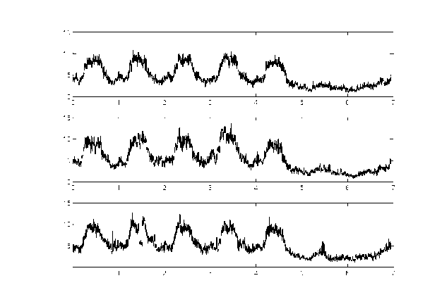
Figure 1: Plot of HTTP operations for three weeks. X axis: day. Y axis: number of operations.
The dataset we use is from a production web server at a large computer company using the collection facility described in [4]. The variable we chose to model is the number of HTTP operations per second that are performed by the web server. Data are collected at a five-minute interval, for a total of 288 intervals in a day.
Figure 1 plots three weeks of HTTP operations. From the plot, we notice that there is an underlying trend for every week. For each workday morning, the HTTP operation increase as people arrive at work. Soon afterwards, the HTTP operations peeks and remains there for most of the day. In late afternoon, values return to lower levels. On weekends, the usage remain low throughout the day.
Clearly, HTTP operations per second is non-stationary in that the mean changes with time-of-day and day-of-week. However, the previous figure suggests that the same non-stationary pattern is present from week to week (or that it changes slowly). Thus, we can view the full process as having a stable mean for each time of the day along with fluctuations that are modeled by a random variable with a zero mean. We treat the means as a separate subpro-cess, which we refer to as the trend subprocess. By subtracting the trend from the original data, we obtain the residual process, which is assumed to be stationary.
Our prediction scheme is structured as follows. First, the trend process is estimated from the original process. Next, the residual process is constructed by subtracting trend from the original process. Then, prediction is done on the residual process. Finally, the trend is added back for the ultimate prediction result. The modeling required to support these steps is divided into two parts: modeling of the non-stationary or trend subprocess and the modeling of the residual subprocess.
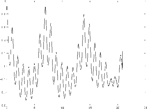
Figure 2: Plot of autocorrelation. X axis: day. Y axis: autocorrelation.
Let Xt denote the process over a week. That is, t ranges over 288 x 7 = 2016 values. We decompose Xt into a trend subprocess and a residual subprocess, i.e.,
where Yt denotes the trend subprocess and XR denotes the residual subprocess. At each time instant t, Yt is deterministic and XR is a random variable. The index t is computed from i, the day of week, and j, the time of day, as follows:
where N is number of samples in a day.
In [8], trend is modeled on a daily basis. The reason why we model the process at a weekly level is indicated by Figure 2, which plots the autocorrelation function of three weeks of data. Note that the strongest correlation exists for data at the interval of a week. This suggests a weekly pattern. Also, in Figure 3, we plotted the spectrum of data, obtained from the Fourier transform of 20 weeks of data. The X axis represents number of cycles that happen in a week. We can notice there are two outstanding peaks away from the origin, at 1 and 7, which correspond to a weekly cycle and a daily cycle. From the spectrum we notice a strong presence of frequency components at the cycle of a week. The components at a daily level ( 7 cycles/week ) is relatively weaker. This justifies our modeling approach at a weekly level is more appropriate.
Figure 3: Spectrum of data. X axis: cycles/week. Y axis: spectral amplitude.
This section addresses the estimation of the trend component Yt in Equation (1). Intuitively, Yt should be a smooth process, much smoother than the original process Xt.
In contrast with [8], our scheme uses only three consecutive weeks of the eight months of data to estimate each Yt. We restrict ourselves to such subsets for several reasons. First, we reduce the dependencies on historical data. This is important since the amount of historical data may be limited due to constraints on disk space, network changes (which makes older data obsolete), and other factors. Second, the trend itself may change over time. There can be numerous factors affecting the trend, such as network upgrades, or large scale changes in work assignments within the company. Usually those factors are not predictable. In our data, for example, HTTP operations per second increases over a period of months. Thus, including more than a few weeks of data may adversely affect the trend model. Thus, we restrict ourselves to three weeks of data.
Figure 4 is the power spectrum density of a week. Since we view the whole process as the superposition of two subprocesses, the trend can be viewed as mainly containing low frequency components, while the high frequency parts correspond to the residual process. Thus we use a low pass filter to filter out the high frequency component, then the filtered data are further averaged to obtain the trend. The filter we use is a fourth order Butterworth digital low pass filter with normalized cutoff frequency 0.2. For knowledge about Butterworth filter, see [10].
Here is the algorithm for estimating Yt. Let the impulse response of the low pass filter be h(t). For week i, the data is X\, and the filtered result is Wt\ There is
Figure 4: Power spectrum density plot of a typical weekday. X axis: normalized frequency. Y axis: spectral amplitude.
In [8], the trend model incorporates monthly effects. Further, the trend model assumes that the interaction between time-of-day and day-of-week can be expressed in an additive manner. In essence, this model assumes that patterns for different days in a week should be similar. We refer to this as the daily model of trend.
Our approach, which we refer to as the weekly model, differs from the foregoing. We observe that the interaction of time-of-day and day-of-week effects are not additive. Thus, it makes sense to have a separate interaction term for each time-of-day and day-of-week. Further, the assumption of similar pattern is only acceptable for weekdays. Obviously weekends have very different patterns from that of the weekdays and so cannot be modeled similarly. (Actually the work in [8] only considered weekdays.) Still, the daily model is unable to capture pattern differences between weekdays, except through the mean. While weekly model more accurately reflects the trend process, it has the disadvantage of introducing more parameters.
The effectiveness of the two modeling strategy is compared in Figure 5 and Figure 6 for five work days. The residual process is obtained by using the weekly and daily models on the same length of data (three weeks).
From the comparison we can see the weekly model can better detrend the
where * denotes convolution. Then Yt is estimated as
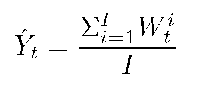
where I is the total number of weeks. In our work, I is 3. Then the process Xt can be detrended by subtracting Yt, i.e.,
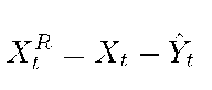
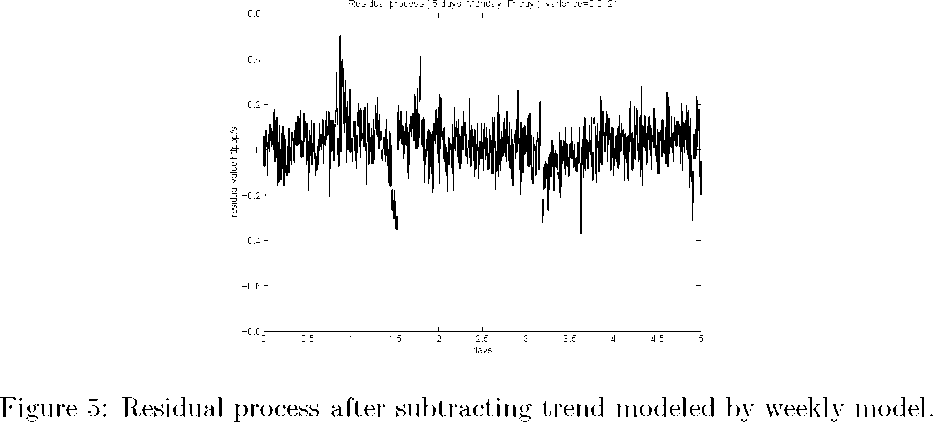

Figure 6: Residual process after subtracting trend modeled by daily model.
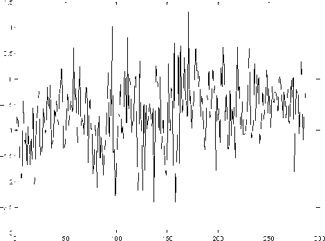
Figure 7: Residual after subtracting trend. X axis: time index in a day. Y axis: HTTP operations after removing the trend.
original process, and the residual process variance is smaller. This is not surprising given the previous discussions.
4 Modeling the Residual Process
This section discusses the modeling of XR, the residual process. The residual process is estimated by subtracting the estimate of Yt from Xt. Figure 7 plots the data of one day after subtracting the trend. Clearly, this plot is more consistent with a stationary process than when the trend is present. However, the data are highly bursty.
We consider predicting the residual process at time t + n. It requires the estimation of its mean and variance. We use an autoregressive (AR) model. AR model is a simple and effective method in time series modeling. It is also adopted in other works analyzing network traffic (e.g., [6, 7]). A second order AR model is used, which is denoted by AR(2). That is,
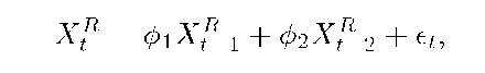
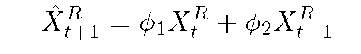
where XR denotes the residual process, and are two AR(2) parameters, and et is the error term, which is assumed to be an independently and identically distributed (i.i.d.) Gaussian random variables with a mean of zero and a variance of a". When XR and XRi are known, XR+i is predicted as
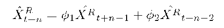
For n step prediction,
This section evaluates the effectiveness of the model developed in the preceding sections. Our focus is XR. Indeed, we treat the Yt process as deterministic. Thus, the evaluation here addresses AR models. We use the characteristic function of the AR model to assess the limits of prediction using an AR model. Following this, we study in detail the error terms in the AR model, et.
Here, we study the accuracy of an n step prediction. As we predict further into the future, the variance of the prediction error increases, which can be analyzed in a straightforward manner. As is commonly used in the literature (as in [8]), the AR(2) model can be expressed as
where Ai and A2 are roots of equation 1 — 4>iB — ^2B2 = 0. For the AR process to be stable, we require |A1| < 1, |A2| < 1. Note that XR is Gaussian since it is a linear combination of Gaussian random variables. We define
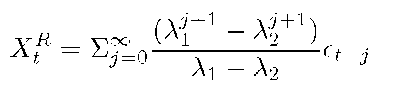
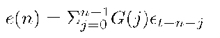
Then, XtR is expressed as
XR = j G(j>t-j. (12)
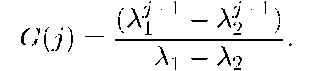
The coefficient function G(j) is called the characteristic function of the AR model, which can characterizes how much the future can be predicted based on current values. When G(j) is small, the influence of et-j- is small. Further, observe that in a stable system, G(j) is an exponentially decreasing function of j. The speed of decay is determined by At. In out data, At's are real values and much smaller than one. The result is a fast decaying characteristic function G(j), as depicted in Figure 8.
Figure 8 plots the characteristic function using values of At estimated from the residuals of one day's data. From our experience, At's are mostly small and G(j) changes little for different days.
As noticed in the figure, G(j) falls below 0.1 after just five steps (j = 5). This indicates our ability to predict the residual process is very limited.
We need to add back the subtracted trend term Yt to get the final prediction value
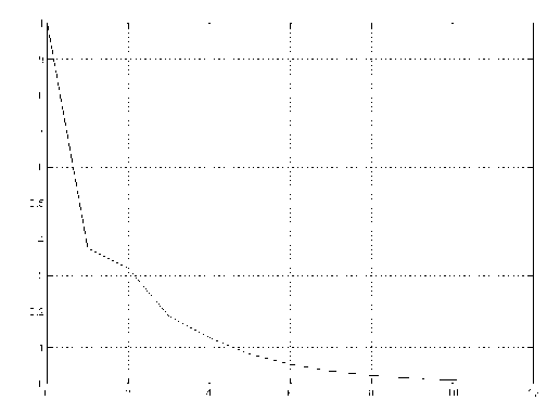
Figure 8: A typical characteristic function of an AR(2) model. X axis: j. Y axis: G(j).
For the purpose of prediction, XtRn can be expressed as
The first term on the right-hand-side is based on future values from t+1 through t + n — 1. The second term is determined by the present and past data at time t,t — 1, t — 2,... . For an n step prediction, the first term is unknown. We estimate it by using the expected value of et+n_j, 0 < j < n, which is 0. Thus, XtRn is estimated as
and the prediction error is
The error term is a linear combination of zero mean i.i.d. Gaussian random variables. Thus, it is also Gaussian with mean of zero, and variance
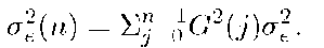
For an n step prediction, from Equation 16, the error variance is determined by two factors- the error variance of one step prediction a", and characteristic function G. For an AR process, the variance of et is fixed. Then G(j) determines how error variance increases with n. For the characteristic function plotted in Figure 8, we see that the influence of past values is negligible after just five steps. That is, when we predict more than five steps ahead, the predicted value is close to zero, and the error variance is large.
To elaborate on the last point, we introduce the notion of predictable steps for an AR model. The intention is to quantify the number of steps into the
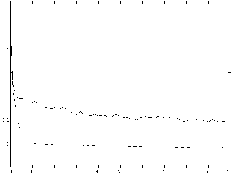
Figure 9: Comparison of autocorrelation function. '-': residual process. '-': AR process. X axis: lag. Y axis: autocorrelation.
future for which it is meaningful to do prediction. Let s2(t + n) be the energy of XtRn, where s2(t + n) = (XtRn)2. The ratio between s2(t + n) and ^(n) provides insight into the quality of an n step prediction at time t. This ratio is
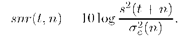
This expression has the form of a signal-to-noise ratio. Here, the signal is the predicted value, and the noise is the prediction variance. From the discussion of the characteristic function, we know that as AR predictions extend further into the future, the predicted value of an AR process decreases, and its variance increases. Thus, snr is a decreasing function of n.
The foregoing discussion suggests that snr can be used as a stopping rule for AR-based prediction. When snr drops below a specified threshold, AR-based prediction should not continue. However, for our application, we can still use the trend to give us information about the future. We can set XR_n to 0, so that Xt+n = Yt+n. Thus, for larger n, we only consider the trend component when making a prediction.
We briefly consider a second issue for using an AR model. This relates to long-range dependence in the data. Others have noted that network traffic exhibits long range dependence (e.g., [11]). Figure 9 plots the autocorrelation function of the residual process in our data and the autocorrelation function of the AR process using parameters estimated from the residual process.
We see that for large lags, the autocorrelation of AR process decays exponentially fast, while the correlation of data decays at a much slower speed, exhibiting long-range dependence. This failure to capture long range dependencies is a drawback of the AR model and affects its ability to predict the residual process, especially for larger n.
5.3 Probability of Violating a Threshold
An important application of predictive models for proactive management is estimating the probability of violating a threshold (e.g., as in [8]). This is accomplished by estimating the mean and variance of a future observation and then using the assumption of Gaussian error terms to estimate the probability of violating a threshold.
To provide more details, we consider an n step prediction. The random variable Xt+n can be expressed as Xt+n = Xt+n + et+n, where Xt+n is given by
which is the summation of the trend and predicted value of the residual process.
The distribution of the random variable Xt+n is determined by the distribution of et+n, which is assumed to be a zero mean Gaussian random variable. Then Xt+n is also a Gaussian random variable with its mean given by Equation 18, and variance by Equation 16.
We consider a threshold T for which we want to estimate the probability that Xt+n > T. As in [8], we transform T into units of XR_n, which results in a time-varying threshold whose value is tht+n at time t + n. Thus, it suffices to estimate probability that XtRn > tht+n given that the mean of Xt+n is Xt+n and its variance is a". Let Pt(n) denote this probability. Then,
where $(^)is the cumulative distribution function of Gaussian distribution N(0,1).
5.4 Distribution of Error Term
The above analysis is based on the assumption of a Gaussian distribution for the error term. However, the error term distribution may not be Gaussian. Figure 10 is the quantile-quantile plot of one step prediction error distribution against that of Gaussian. The straight line is Gaussian, while the thick line is for the error term. We notice considerable differences in the tail behavior of the two distributions in that the tail of the prediction error is "fatter" than that of the Gaussian. That is, when the threshold falls on the tail, the Gaussian assumption over estimates the probability of a threshold violation. Also from the quantile plot, the prediction error distribution copes with that of Gaussian for most of the parts except the tail. In reality we are usually concerned with cases when the probability of threshold violation is large enough and tend to neglect small probabilities. Then the error in the tail is not a major concern. In that sense, employing a Gaussian assumption is an acceptable approximation for the error distribution.
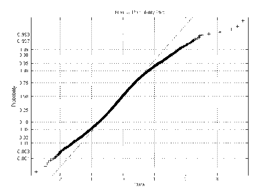
Figure 10: Quantile-quantile plot of the prediction error.
Proactive management can allow service providers to take action in advance of service disruptions. However, being proactive requires a capability to predict system behavior. This paper investigates issues related to prediction in the context of web server data.
Our focus has been to extend the work in [8] in several ways. Our extensions include: we enhance the trend model by employing filtering techniques and by considering the trend over a shorter time span; we examine assumptions underlying the stationary component, including the assumption of a Gaussian distribution for the error terms in the residual process; the limits of prediction using AR models is analyzed; we show long-range dependence remains in the data after the trend and stationary components are removed, which poses challenges for prediction.
We see a number of areas that should be investigated more fully. A fundamental issue is the burstiness and non-stationary of the data. Our AR(2) model is unable to deal with long range dependence. A model capable of dealing with long range dependence may improve the prediction precision. On the other hand, we model the trend as a fixed process. The prediction performed on the residual process limits prediction quality, constrained by the ability of AR model and the noisy nature of the residual process. We may improve our prediction by predicting the trend instead, which is much less noisy than the residual process. This requires an adaptive trend model to capture the trend evolution. Sometimes, the prediction on the trend may be of more interests for network managers.
We wish to thank Sheng Ma for helpful comments and stimulating discussions.
[1] George E.P. Box, Gwilym M. Jenkins, Time Series Forecasting and Control, Prentice Hall, 1976.
[2] M.Dutta, Executive Editor, Economics, Econometrics and the Links, North Holland, 1995.
[3] Andrei S.Monin, Weather Forecasting as a Problem in Physics, MIT Press, Cambridge, MA 1972.
[4] Adrian Cochcroft, "Watching Your Web Servers", SunWorld OnLine, http://www.sunworld.com/swol-03-1996/swol-03-perf.html.
[5] C.S.Hood, C. Ji, "Proactive Network Fault Detection", Proceedings of IN-FOCOM, Kobe, Japan, 1997.
[6] P. Hoogenboom, J. Lepreau, "Computer System Performance Detection Using Time Series Models", Proc. of the Summer USENIX Conference, pp. 15-32, 1993.
[7] Marina Throttan, C. Ji, "Adaptive Thresholding for Proactive Network Problem Detection," Third IEEE International Workshop on Systems Management, pp. 108-116, Newport, Rhode Island, April, 1998.
[8] Joseph L. Hellerstein, Fan Zhang, P.Shahabuddin, "An Approach to Predictive Detection for Service Management," Symposium on Integrated Network Management, 1999.
[9] Thomas Kailath, Kalman Filtering: Theory and Pracitce, Prentice Hall, 1993.
[10] Bernard Widrow, Samuel D.Strearns, Adaptive Signal Processing, Prentice Hall, 1985.
[11] W. E. Leland, M. S. Taqqu, Walter Willinger, D. V. Wilson, "On the Self-Similarity Nature of Ethernet Traffic (Extended Version)", IEEE Trans. on Networking, Vol. 2, No.1, pp. 1-14, Feb. 1994.