Amit’s Notes about Path-Finding
Amit Patel
Источник: Amit’s Notes about Path-Finding, amitp@cs.stanford.edu
http://theory.stanford.edu/~amitp/GameProgramming/
The problem we’re trying to solve is to get a game object from the starting point to a goal. Pathfinding addresses the problem of finding a good path from the starting point to the goal?avoiding obstacles, avoiding enemies, and minimizing costs (fuel, time, distance, equipment, money, etc.). Movement addresses the problem of taking a path and moving along it. It’s possible to spend your efforts on only one of these. At one extreme, a sophisticated pathfinder coupled with a trivial movement algorithm would find a path when the object begins to move and the object would follow that path, oblivious to everything else. At the other extreme, a movement-only system would not look ahead to find a path (instead, the initial “path” would be a straight line), but instead take one step at a time, considering the local environment at every point. Best results are achieved by using both pathfinding and movement algorithms.
Introduction
Movement for a single object seems easy. Pathfinding is complex. Why bother with pathfinding? Consider the following situation:

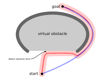
The unit is initially at the bottom of the map and wants to get to the top. There is nothing in the area it scans (shown in pink) to indicate that the unit should not move up, so it continues on its way. Near the top, it detects an obstacle and changes direction. It then finds its way around the “U”-shaped obstacle, following the red path. In contrast, a pathfinder would have scanned a larger area (shown in light blue), but found a shorter path (blue), never sending the unit into the concave shaped obstacle.
You can however extend a movement algorithm to work around traps like the one shown above. Either avoid creating concave obstacles, or mark their convex hulls as dangerous (to be entered only if the goal is inside):
Pathfinders let you look ahead and make plans rather than waiting until the last moment to discover there’s a problem. There’s a tradeoff between planning with pathfinders and reacting with movement algorithms. Planning generally is slower but gives better results; movement is generally faster but can get stuck. If the game world is changing often, planning ahead is less valuable. I recommend using both: pathfinding for big picture, slow changing obstacles and long paths; and movement for local area, fast changing, and short paths.
Algorithms
The pathfinding algorithms from computer science textbooks work on graphs in the mathematical sense?a set of vertices with edges connecting them. A tiled game map can be considered a graph with each tile being a vertex and edges drawn between tiles that are adjacent to each other:

For now, I will assume that we’re using two-dimensional grids. Later on, I’ll discuss how to build other kinds of graphs out of your game world.
Most pathfinding algorithms from AI or Algorithms research are designed for arbitrary graphs rather than grid-based games. We’d like to find something that can take advantage of the grid nature of the map. There are some things we consider common sense, but that algorithms don’t understand. For example, we know something about directions: we know that in general, as two things get farther apart, it will take a longer to move from one to the other; and we know that there aren’t any secret wormholes that let you teleport from one spot on the map to another. (Well, I assume there aren’t any; if there are, it becomes very hard to find a good path because you don’t know where to look first.)
Dijkstra’s Algorithm and Best-First-Search
Dijkstra’s algorithm works by visiting vertices in the graph starting with the object’s starting point. It then repeatedly examines the closest not-yet-examined vertex, adding its vertices to the set of vertices to be examined. it expands outwards from the starting point until it reaches the goal. Dijkstra’s algorithm is guaranteed to find a shortest path from the starting point to the goal, as long as none of the edges have a negative cost. (I write “a shortest path” because there are often multiple equivalently-short paths.) In the following diagram, the pink square is the starting point, the blue square is the goal, and the teal areas show what areas Dijkstra’s algorithm scanned. The lightest teal areas are those farthest from the starting point, and thus form the “frontier” of exploration:

The Greedy Best-First-Search algorithm works in a similar way, except that it has some estimate (called a heuristic) of how far from the goal any vertex is. Instead of selecting the vertex closest to the starting point, it selects the vertex closest to the goal. (Greedy) Best-First-Search is not guaranteed to find a shortest path. However, it runs much quicker than Dijkstra’s algorithm because it uses the heuristic function to guide its way towards the goal very quickly. For example, if the goal is to the south of the starting position, Best-First-Search will tend to focus on paths that lead southwards. In the following diagram, yellow represents those nodes with a high heuristic value (high cost to get to the goal) and black represents nodes with a low heuristic value (low cost to get to the goal). It shows that Best-First-Search can find paths very quickly compared to Dijkstra’s algoritm:
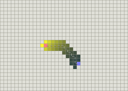
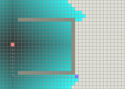
However, both of these examples illustrate the simplest case?when the map has no obstacles, and the shortest path really is a straight line. Let’s consider the concave obstacle as described in the previous section. Dijkstra’s algorithm works harder but is guaranteed to find a shortest path:
Best-First-Search on the other hand does less work but its path is clearly not as good:
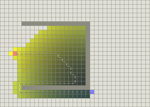
The trouble is that Greedy Best-First-Search is “greedy” and tries to move towards the goal even if it’s not the right path. Since it only considers the cost to get to the goal and ignores the cost of the path so far, it keeps going even if the path it’s on has become really long.
Wouldn’t it be nice to combine the best of both? A* was developed in 1968 to combine heuristic approaches like Best-First-Search and formal approaches like Dijsktra’s algorithm. It’s a little unusual in that heuristic approaches usually give you an approximate way to solve problems without guaranteeing that you get the best answer. However, A* is built on top of the heuristic, and although the heuristic itself does not give you a guarantee, A* can guarantee a shortest path.
The A* Algorithm
I will be focusing on the A* Algorithm. A* is the most popular choice for pathfinding, because it’s fairly flexible and can be used in a wide range of contexts.
A* is like other graph-searching algorithms in that it can potentially search a huge area of the map. It’s like Dijkstra’s algorithm in that it can be used to find a shortest path. It’s like Greedy Best-First-Search in that it can use a heuristic to guide itself. In the simple case, it is as fast as Best-First-Search:

In the example with a concave obstacle, A* finds a path as good as what Dijkstra’s algorithm found:
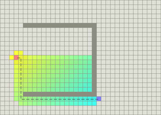
The secret to its success is that it combines the pieces of information that Dijkstra’s algorithm uses (favoring vertices that are close to the starting point) and information that Best-First-Search uses (favoring vertices that are close to the goal). In the standard terminology used when talking about A*, g(n) represents the cost of the path from the starting point to any vertex n, and h(n) represents the heuristic estimated cost from vertex n to the goal. In the above diagrams, the yellow (h) represents vertices far from the goal and teal (g) represents vertices far from the starting point. A* balances the two as it moves from the starting point to the goal. Each time through the main loop, it examines the vertex n that has the lowest f(n) = g(n) + h(n).