APPLYING NEURAL NETWORK MODELS TO PREDICTION AND DATA ANALYSIS IN METEOROLOGY AND OCEANOGRAPHY
Автор: Christopher R. Williams
Источник: Journal of Atmospheric and Oceanic Technology, Volume 79, Issue 9 (September 1998) pp. 1855-1870
Abstarct
Empirical or statistical methods have been introduced into meteorology and oceanography in four distinct stages:
1) linear regression (and correlation),
2) principal component analysis (PCA),
3) canonical correlation analysis, and recently 4) neural network (NN) models. Despite the great popularity of the NN models in many fields, there are three obstacles to adapting the NN method to meteorology–oceanography, especially in large-scale, low-frequency studies:
(a) nonlinear instability with short data records, (b) large spatial data fields, and (c) difficulties in interpreting the nonlinear NN results. Recent research shows that these three obstacles can be overcome. For obstacle (a), ensemble averaging was found to be effective in controlling nonlinear instability. For (b), the PCA method was used as a prefilter for compressing the large spatial data fields. For (c), the mysterious hidden layer could be given a phase space interpretation, and spectral analysis aided in understanding the nonlinear NN relations. With these and future improvements, the nonlinear NN method is evolving to a versatile and powerful technique capable of augmenting traditional linear statistical methods in data analysis and forecasting; for example, the NN method has been used for El Niño prediction and for nonlinear PCA. The NN model is also found to be a type of variational (adjoint) data assimilation, which allows it to be readily linked to dynamical models under adjoint data assimilation, resulting in a new class of hybrid neural–dynamical models.
1.Introduction
The introduction of empirical or statistical methods into meteorology and oceanography can be broadly classified as having occurred in four distinct stages: 1) Regression (and correlation analysis) was invented by Galton (1885) to find a linear relation between a pair of variables x and z. 2) With more variables, the principal component analysis (PCA), also known as the empirical orthogonal function (EOF) analysis, was introduced by Pearson (1901) to find the correlated patterns in a set of variables x1 , . . ., xn. It became popular in meteorology only after Lorenz (1956) and was later introduced into physical oceanography in the mid-1970s. 3) To linearly relate a set of variables x1, . . ., xn to another set of variables z1 , . . ., zm, the canonical correlation analysis (CCA) was invented by Hotelling (1936), and became popular in meteorology and oceanography after Barnett and Preisendorfer (1987). It is remarkable that in each of these three stages, the technique was first invented in a biological–psychological field, long before its adaptation by meteorologists and oceanographers many years or decades later. Not surprisingly, stage 4, involving the neural network (NN) method, which is just starting to appear in meteorology–oceanography, also had a biological–psychological origin, as it developed from investigations into the human brain function. It can be viewed as a generalization of stage 3, as it nonlinearly relates a set of variables x1 . . ., xn to an-
other set of variables z1, . . ., zm.
The human brain is one of the great wonders of nature-even a very young child can recognize people and objects much better than the most advanced artificial intelligence program running on a supercomputer. The brain is vastly more robust and fault tolerant than a computer. Though the brain cells are continually dying off with age, the person continues to recognize friends last seen years ago. This robustness is the result of the brain’s massively parallel computing structure, which arises from the neurons being interconnected by a network. It is this parallel computing structure that allows the neural network, with typical neuron “clock speeds” of a few milliseconds, about a millionth that of a computer, to outperform the computer in vision, motor control, and many other tasks.
Fascinated by the brain, scientists began studying logical processing in neural networks in the 1940s (McCulloch and Pitts 1943). In the late 1950s and early 1960s, F. Rosenblatt and B. Widrow independently investigated the learning and computational capability of neural networks (Rosenblatt 1962; Widrow and Sterns 1985). The perceptron model of Rosenblatt consists of a layer of input neurons, interconnected to an output layer of neurons. After the limits of the perceptron model were found (Minsky and Papert 1969), interests in neural network computing waned, as it was felt that neural networks (also called connectionist models) did not offer any advantage over conventional computing methods.
While it was recognized that the perceptron model was limited by having the output neurons linked directly to the neurons, the more interesting problem of having one or more “hidden” layers of neurons (Fig. 1) between the input and output layer was mothballed due to the lack of an algorithm for finding the weights in terconnecting the neurons. The hiatus ended in the second half of the 1980s, with the rediscovery of the back-propagation algorithm (Rumelhart et al. 1986), which successfully solved the problem of finding the weights in a model with hidden layers. Since then, NN research rapidly became popular in artificial intelligence, robotics, and many other fields (Crick 1989). Neural networks were found to outperform the linear Box–Jenkins models (Box and Jenkins 1976) in forecasting time series with short memory and at longer lead times (Tang et al. 1991). During 1991–92, the Santa Fe Institute sponsored the Santa Fe Time Series Prediction and Analysis Competition, where all prediction methods were invited to forecast several time series. For every time series in the competition, the winner turned out to be an NN model (Weigend and Gershenfeld 1994).
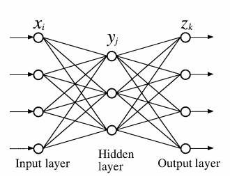
FIG. 1. A schematic diagram illustrating a neural network model with one hidden layer of neurons between the input layer and the output layer. For a feed-forward network, the information only flows forward starting from the input neurons
Among the countless applications of NN models, pattern recognition provides many intriguing examples; for example, for security purposes, the next generation of credit cards may carry a recorded electronic image of the owner. Neural networks can now correctly verify the bearer based on the recorded image, a nontrivial task as the illumination, hair, glasses, and mood of the bearer may be very different from those in the recorded image (Javidi 1997). In artificial speech, NNs have been successful in pronouncing English text (Sejnowski and Rosenberg 1987). Also widely applied to financial forecasting (Trippi and Turban 1993; Gately 1995; Zirilli 1997), NN models are now increasingly being used by bank and fund managers for trading stocks, bonds, and foreign currencies. There are well over 300 books on artificial NNs in the subject guide to Books in Print, 1996-97 (published by R.R. Bowker), including some good texts (e.g., Bishop 1995; Ripley 1996; Rojas 1996).
By now, the reader must be wondering why these ubiquitous NNs are not more widely applied to meteorology and oceanography. Indeed, the purpose of this paper is to examine the serious problems that can arise when applying NN models to meteorology and oceanography, especially in large-scale, low frequency studies, and the attempts to resolve these problems. Section 2 explains the difficulties encountered with NN models, while section 3 gives a basic introduction to NN models. Sections 4–6 examine various solutions to overcome the difficulties mentioned in section 2. Section 7 applies the NN method to El Niño forecasting, while section 8 shows how the NN can be used as nonlinear PCA. The NN model is linked to variational (adjoint) data assimilation in section 9.
2.Difficulties in applying neural networks to meteorology-oceanography
Elsner and Tsonis (1992) applied the NN method to forecasting various time series, and comparing with forecasts by autoregressive (AR) models. Unfortunately, because of the computer bug noted in their corrigendum, the advantage of the NN method was not as conclusive as in their original paper. Early attempts to use neural networks for seasonal climate forecasting were also at best of mixed success (Derr and Slutz 1994; Tang et al. 1994), showing little evidence that exotic, nonlinear NN models could beat standard linear statistical methods such as the CCA method (Barnett and Preisendorfer 1987; Barnston and Ropelewski 1992; Shabbar and Barnston 1996) or its variant, the singu- lar value decomposition (SVD) method (Bretherton et al. 1992), or even the simpler principal oscillation pattern (POP) method (Penland 1989; von Storch et al. 1995; Tang 1995).
There are three main reasons why NNs have difficulty being adapted to meteorology and oceanography: (a) nonlinear instability occurs with short data records, (b) large spatial data fields have to be dealt with, and (c) the nonlinear relations found by NN models are far less comprehensible than the linear relations found by regression methods. Let us examine each of these difficulties.
(a)Relative to the timescale of the phenomena one is trying to analyze or forecast, most meteorological and oceanographic data records are short, especially for climate studies. While capable of modeling the nonlinear relations in the data, NN models have many free parameters. With a short data record, the problem of solving for many parameters is ill conditioned; that is, when searching for the global minimum of the cost function associated with the problem, the algorithm is often stuck in one of the numerous local minima surrounding the true global minimum (Fig. 2). Such an NN could give very noisy or completely erroneous forecasts, thus performing far worse than a simple linear statistical model. This situation is analogous to that found in the early days of numerical weather pre- diction, where the addition of the nonlinear advective terms to the governing equations, instead of improving the forecasts of the linear models, led to disastrous nonlinear numerical instabilities (Phillips 1959), which were overcome only after extensive research on how to discretize the advective terms correctly. Thus the challenge for NN models is how to control nonlinear instability, with only the relatively short data records available.
(b)Meteorological and oceanographic data tend to cover numerous spatial grids or stations, and if each station serves as an input to an NN, then the NN will have a very large number of inputs and associated weights. The optimal search for many weights over the relatively short temporal records would be an ill-conditioned problem. Hence, even though there had been some success with NNs in seasonal forecasting using a small number of predictors (Navone and Ceccatto 1994; Hastenrath et al. 1995), it was unclear how the method could be generalized to large data fields in the manner of CCA or SVD methods.
(c)The interpretation of the nonlinear relations found by an NN is not easy. Unlike the parameters from a linear regression model, the weights found by an NN model are nearly incomprehensible. Furthermore, the “hidden” neurons have always been a mystery.
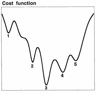
FIG. 2. A schematic diagram illustrating the cost function sur- face, where depending on the starting condition, the search algo- rithm often gets trapped in one of the numerous deep local minima. The local minima labeled 2, 4, and 5 are likely to be reasonable local minima, while the minimum labeled 1 is likely to be a bad one (in that the data was not well fitted at all). The minimum labeled 3 is the global minimum, which could correspond to an overfitted solution (i.e., fitted closely to the noise in the data) and may, in fact, be a poorer solution than the minima labeled 2, 4, and 5.
Over the last few years, the University of British Columbia Climate Prediction Group has been trying to overcome these three obstacles. The purpose of this paper is to show how these obstacles can be overcome: For obstacle a, ensemble averaging was found to be effective in controlling nonlinear instability. Various penalty, pruning, and nonconvergent methods also helped. For b, the PCA method was used to greatly reduce the dimension of the large spatial data fields. For c, new measures and visualization techniques helped in understanding the nonlinear NN relations and the mystery of the hidden neurons. With these improvements, the NN approach has evolved to a tech- nique capable of augmenting the traditional linear sta- tistical methods currently used.
Since the focus of this review is on the application of the NN method to low-frequency studies, we will only briefly mention some of the higher-frequency applications. As the problem of short data records is no longer a major obstacle in higher-frequency appli- cations, the NN method has been successfully used in areas such as satellite imagery analysis and ocean acoustics (Lee et al. 1990; Badran et al. 1991; IEEE 1991; French et al. 1992; Peak and Tag 1992; Bankert 1994; Peak and Tag 1994; Stogryn et al. 1994; Krasnopolsky et al. 1995; Butler et al. 1996; Marzban and Stumpf 1996; Liu et al. 1997).
3.Neural network models
To keep within the scope of this paper, we will limit our survey of NN models to the feed-forward neural network. Figure 1 shows a network with one hidden layer, where the jth neuron in this hidden layer is assigned the value yj , given in terms of the input values xi by
 (1)
(1)
where wij and bj are the weight and bias parameters, respectively, and the hyperbolic tangent function is used as the activation function (Fig. 3). Other functions besides the hyperbolic tangent could be used for the activation function, which was designed originally to simulate the firing or nonfiring of a neuron upon re- ceiving input signals from its neighbors. If there are additional hidden layers, then equations of the same form as (1) will be used to calculate the values of the next layer of hidden neurons from the current layer of neurons. The output neurons zk are usually calculated by a linear combination of the neurons in the layer just before the output layer, that is,
 (2)
(2)
To construct a NN model for forecasting, the predic- tor variables are used as the input, and the predictands (either the same variables or other variables at some lead time) as the output. With zdk denoting the observed data, the NN is trained by finding the optimal values of the weight and bias parameters (wij , w ~ jk , bj , and b ~ k ), which will minimize the cost function:
 (3)
(3)
where the rhs of the equation is simply the sum- squared error of the output. The optimal parameters can be found by a back-propagation algorithm (Rumelhart et al. 1986; Hertz et al. 1991). For the reader familiar with variational data assimilation meth- ods, we would point out that this back propagation is equivalent to the backward integration of the adjoint equations in variational assimilation (see section 9).
The back-propagation algorithm has now been perceded by more efficient optimization algorithms,
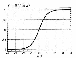
FIG. 3. The activation function y = tanh(wx + b), shown with b = 0. The neuron is activated (i.e., outputs a value of nearly +1) when the input signal x is above a threshold; otherwise, it remains inactive (with a value of around −1). The location of the thresh- old along the x axis is changed by the bias parameter b and the steepness of the threshold is changed by the weight w.
such as the conjugate gradient method, simulated annealing, and genetic algorithms (Hertz et al. 1991). Once the optimal parameters are found, the training is finished, and the network is ready to perform fore- casting with new input data. Normally the data record is divided into two, with the first piece used for net- work training and the second for testing forecasts. Due to the large number of parameters and the great flex- ibility of the NN, the model output may fit the data very well during the training period yet produce poor forecasts during the test period. This results from overfitting; that is, the NN fitted the training data so well that it fitted to the noise, which of course resulted in the poor forecasts over the test period (Fig. 4). An NN model is usually capable of learning the signals in the data, but as training progresses, it often starts learning the noise in the data; that is, the forecast error of the model over the test period first decreases and then increases as the model starts to learn the noise in the training data. Overfitting is often a serious prob- lem with NN models, and we will discuss some solu- tions in the next section.
Consider the special case of a NN with no hidden layers—inputs being several values of a time series, output being the prediction for the next value, and the input and output layers connected by linear activation functions. Training this simple network is then equiva- lent to determining an AR model through least squares regression, with the weights of the NN corresponding to the weights of the AR model. Hence the NN model reduces to the well-known AR model in this limit.
In general, most NN applications have only one or two hidden layers, since it is known that to approxi- mate a set of reasonable functions f k ({xi }) to a given accuracy, at most two hidden layers are needed (Hertz et al. 1991, 142). Furthermore, to approximate continu- ous functions, only one hidden layer is enough (Cybenko 1989; Hornik et al. 1989). In our models for forecasting the tropical Pacific (Tangang et al. 1997; Tangang et al. 1998a; Tangang et al. 1998b; Tang et al. 1998, manuscript submitted to J. Climate, hereafter THMT), we have not used more than one hidden layer. There is also an interesting distinction between the non- linear modeling capability of NN models and that of polynomial expansions. With only a few parameters, the polynomial expansion is only capable of learning low-order interactions. In contrast, even a small NN is fully nonlinear and is not limited to learning low- order interactions. Of course, a small NN can learn only a few interactions, while a bigger one can learn more.
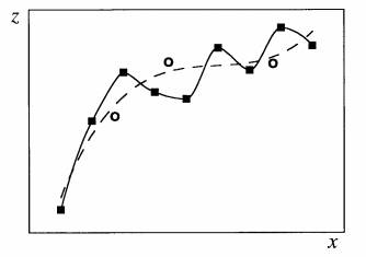
FIG. 4. A schematic diagram illustrating the problem of overfitting: The dashed curve illustrates a good fit to noisy data (indicated by the squares), while the solid curve illustrates overfitting, where the fit is perfect on the training data (squares) but is poor on the test data (circles). Often the NN model begins by fitting the training data as the dashed curve, but with further iterations, ends up overfitting as the solid curve.
When forecasting at longer lead times, there are two possible approaches. The iterated forecasting ap- proach trains the network to forecast one time step forward, then use the forecasted result as input to the same network for the next time step, and this process is iterated until a forecast for the nth time step is obtained. The other is the direct or “jump” forecast approach, where a network is trained for forecasting at a lead time of n time steps, with a different network for each value of n. For deterministic chaotic systems, iterated forecasts seem to be better than direct forecasts (Gershenfeld and Weigend 1994). For noisy time series, it is not clear which approach is better. Our experience with climate data suggested that the direct forecast approach is better. Even with “clearning” and continuity constraints (Tang et al. 1996), the iterated forecast method was unable to prevent the forecast errors from being amplified during the iterations.
4.Nonlinear instability
Let us examine obstacle a; that is, the application of NNs to relatively short data records leads to an ill- conditioned problem. In this case, as the cost function is full of deep local minima, the optimal search would likely end up trapped in one of the local minima (Fig. 2). The situation gets worse when we either (i) make the NN more nonlinear (by increasing the num- ber of neurons, hence the number of parameters), or (ii) shorten the data record. With a different initializa- tion of the parameters, the search would usually end up in a different local minimum.
A simple way to deal with the local minima prob- lem is to use an ensemble of NNs, where their param- eters are randomly initialized before training. The individual NN solutions would be scattered around the global minimum, but by averaging the solutions from the ensemble members, we would likely obtain a bet- ter estimate of the true solution. Tangang et al. (1998a) found the ensemble approach useful in their forecasts of tropical Pacific sea surface temperature anomalies (SSTA).
An alternative ensemble technique is “bagging” (abbreviated from bootstrap aggregating) (Breiman 1996; THMT). First, training pairs, consisting of the predictor data available at the time of a forecast and the forecast target data at some lead time, are formed. The available training pairs are separated into a train- ing set and a forecast test set, where the latter is re- served for testing the model forecasts only and is not used for training the model. The training set is used to generate an ensemble of NN models, where each member of the ensemble is trained by a subset of the training set. The subset is drawn at random with replacement from the training set. The subset has the same number of training pairs as the training set, where some pairs in the training set appear more than once in the subset, and about 37% of the training pairs in the training set are unused in the subset. These unused pairs are not wasted, as they are used to deter- mine when to stop training. To avoid overfitting, THMT stopped training when the error variance from applying the model to the set of “unused” pairs started to increase. By averaging the output from all the in- dividual members of the ensemble, a final output is obtained.
We found ensemble averaging to be most effective in preventing nonlinear instability and overfitting. However, if the individual ensemble members are se- verely overfitting, the effectiveness of ensemble av- eraging is reduced. There are several ways to prevent overfitting in the individual NN models of the en- semble, as presented below.
Stopped training” as used in THMT is a type of nonconvergent method, which was initially viewed with much skepticism as the cost function does not in general converge to the global minimum. Under the enormous weight of empirical evidence, theorists have finally begun to rigorously study the properties of stopped training (Finnoff et al. 1993). Intuitively, it is “Stopped training” as used in THMT is a type of nonconvergent method, which was initially viewed with much skepticism as the cost function does not in general converge to the global minimum. Under the enormous weight of empirical evidence, theorists have finally begun to rigorously study the properties of stopped training (Finnoff et al. 1993). Intuitively, it is Another approach to prevent overfitting is to penalize the excessive parameters in the NN model. The ridge regression method (Chauvin, 1990; Tang et al. 1994; Tangang et al. 1998a, their appendix) modifies the cost function in (3) by adding weight penalty terms, that is,
![]() (4)
(4)
with c1 , c2 positive constants, thereby forcing unimpor- tant weights to zero.
Another alternative is network pruning, where insignificant weights are removed. Such methods have oxymoronic names like “optimal brain damage” (Le Cun et al. 1990). With appropriate use of penalty and pruning methods, the global minimum solution may be able to avoid overfitting. A comparison of the effectiveness of nonconvergent methods, penalty methods, and pruning methods is given by Finnoff et al. (1993).
In summary, the nonlinearity in the NN model introduces two problems: (i) the presence of local minima in the cost function, and (ii) overfitting. Let D be the number of data points and P the number of parameters in the model. For many applications of NN in robotics and pattern recognition, there is almost an unlimited amount of data, so that D >> P, whereas in contrast, D ~ P in low-frequency meteorological– oceanographic studies. The local minima problem is present when D >> P, as well as when D ~ P. However, overfitting tends to occur when D ~ P but not when D >> P. Ensemble averaging has been found to be effective in helping the NNs to cope with local minima and overfitting problems.
5.Prefiltering the data fields
Let us now examine obstacle b, that is, the spatially large data fields. Clearly if data from each spatial grid is to be an input neuron, the NN will have so many parameters that the problem becomes ill conditioned. We need to effectively compress the input (and out- put) data fields by a prefiltering process. PCA analy- sis is widely used to compress large data fields (Preisendorfer 1988).
In the PCA representation, we have
![]() (5)
(5)
and
![]() (6)
(6)
where en and an are the nth mode PCA and its time coefficient, respectively, with the PCAs forming an orthonormal basis. PCA maximizes the variance of a1 (t) and then, from the residual, maximizes the vari- ance of a2 (t), and so forth for the higher modes, under the constraint of orthogonality for the {en }. If the origi- nal data xi (i = 1, . . . , I) imply a very large number of input neurons, we can usually capture the main vari- ance of the input data and filter out noise by using the first few PCA time series an (n = 1, . . ., N), with N << I, thereby greatly reducing the number of input neu- rons and the size of the NN model.
In practice, we would need to provide information on how the {an } has been evolving in time prior to mak- ing our forecast. This is usually achieved by provid- ing {an (t)}, {an (t−∆t)}, . . ., {an (t−m∆t)}, that is, some of the earlier values of {an }, as input. Compression of input data in the time dimension is possible with the extended PCA or EOF (EPCA or EEOF) method (Weare and Nasstrom 1982; Graham et al. 1987).
In the EPCA analysis, copies of the original data matrix Xij = xi (t j ) are stacked with time lag τ into a larger matrix X′,
![]() (7)
(7)
where the superscript T denotes the transpose and Xij+nτ = xi (t j + nτ). Applying the standard PCA analysis to X′ yields the EPCAs, with the corresponding time se- ries {an ′}, which because time-lag information has al- ready been incorporated into the EPCAs, could be used instead of {an (t)}, {an (t − ∆t)}, . . . {an (t − m∆t)} from the PCA analysis, thereby drastically reducing the number of input neurons.
This reduction in the input neurons by EPCAs comes with a price, namely the time-domain filtering automatically associated with the EPCA analysis, which results in some loss of input information. Monahan et al. (1998, manuscript submitted to Atmos.–Ocean) found that the EPCAs could become degenerate if the lag τ was close to the integral timescale of standing waves in the data. While there are clearly trade-offs between using PCAs and using EPCAs, our experiments with forecasting the tropical Pacific SST found that the much smaller networks re- sulting from the use of EPCAs tended to be less prone to overfitting than the networks using PCAs.
We are also studying other possible prefiltering processes. Since CCA often uses EPCA to prefilter the predictor and predictand fields (Barnston and Ropelewski 1992), we are investigating the possibil- ity of the NN model using the CCA as a prefilter, that is, using the CCA modes instead of the PCA or EPCA modes. Alternatively, we may argue that all these prefilters are linear processes, whereas we should use a nonlinear prefilter for a nonlinear method such as NN. We are investigating the possibility of using NN mod- els as nonlinear PCAs to do the prefiltering (section 8).
6.Interpreting the NN model
We now turn to obstacle c, namely, the great diffi- culty in understanding the nonlinear NN model results. In particular, is there a meaningful interpretation of those mysterious neurons in the hidden layer?
Consider a simple NN for forecasting the tropical Pacific wind stress field. The input consists of the first 11 EPCA time series of the wind stress field (from The Florida State University), plus a sine and cosine func- tion to indicate the phase with respect to the annual cycle. The single hidden layer has three neurons, and the output layer the same 11 EPCA time series one month later. As the values of the three hidden neurons can be plotted in 3D space, Fig. 5 shows their trajec- tory for selected years. From Fig. 5 and the trajecto- ries of other years (not shown), we can identify regions in the 3D phase space as the El Niño warm event phase and its precursor phase and the cold event and its pre- cursor. One can issue warm event or cold event fore- casts whenever the system enters the warm event precursor region or the cold event precursor region, re- spectively. Thus the hidden layer spans a 3D phase space for the El Niño–Southern Oscillation (ENSO) system and is, thus, a higher-dimension generalization of the 2D phase space based on the POP method (Tang 1995).
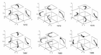
FIG. 5. The values of the three hidden neurons plotted in 3D space for the years 1972, 1973, 1976, 1982, 1983, and 1988. Projections onto 2D planes are also shown. The small circles are for the months from January to December, and the two “+” signs for January and February of the following year. El Niño warm events occurred during 1972, 1976, and 1982, while a cold event occurred in 1988. In 1973 and 1983, the Tropics returned to cooler con- ditions from an El Niño. Notice the similarity between the trajectories during 1972, 1976, and 1982, and during 1973, 1983, and 1988. In years with neither warm nor cold events, the trajectories oscillate randomly near the center of the cube. From these trajectories, we can identify the precursor phase regions for warm events and cold events, which could allow us to forecast these events.
Hence we interpret the NN as a projection from the input space onto a phase space, as spanned by the neu- rons in the hidden layer. The state of the system in the phase space then allows a projection onto the output space, which can be the same input variables some time in the future, or other variables in the future. This interpretation provides a guide for choosing the appro- priate number of neurons in the hidden layer; namely, the number of hidden neurons should be the same as the embedding manifold for the system. Since the ENSO system is thought to have only a few degrees of freedom (Grieger and Latif 1994), we have limited the number of hidden neurons to about 3–7 in most of our NN forecasts for the tropical Pacific, in contrast to the earlier study by Derr and Slutz (1994), where 30 hidden neurons were used. Our approach for gen- erating a phase space for the ENSO attractor with an NN model is very different from that of Grieger and Latif (1994), since their phase space was generated from the model output instead of from the hidden layer. Their approach generated a 4D phase space from using four PCA time series as input and as output, whereas our approach did not have to limit the num- ber of input or output neurons to generate a low- dimensional phase space for the ENSO system.
In many situations, the NN model is compared with a linea model, and one wants to know how nonlinear the NN mode really is. A useful diagnostic tool to measure nonlinearity is spectral analysis (Tangang et al 1998b). Once a network has been trained, we replace the N input signals by artificial sinu soidal signals with frequencies ω1 , ω2 , . . ., ωN, which were care fully chosen so that the nonlin ear interactions of two signals o frequencies ωi and ωj would generate frequencies ωi + ωj and ωi − ωj not equal to any o the original input frequencies The amplitude of a sinusoida signal is chosen so as to yield the same variance as that of the original real input data. The output from the NN with the sinusoidal inputs is spectrally analyzed (Fig. 6). If the NN is basically linear, spec- tral peaks will be found only at the original input fre- quencies. The presence of an unexpected peak at frequency ω′, equaling ωi + ωj or ωi − ωj for some i, j, indicates a nonlinear interaction between the ith and the jth predictor time series. For an overall mea- sure of the degree of nonlinearity of an NN, we can calculate the total area under the output spectrum, ex- cluding the contribution from the original input fre- quencies, and divide it by the total area under the spectrum, thereby yielding an estimate of the portion of output variance that is due to nonlinear interactions. Using this measure of nonlinearity while forecasting the regional SSTA in the equatorial Pacific, Tangang et al. (1998b) found that the nonlinearity of the NN tended to vary with forecast lead time and with geo- graphical location.
7.Forecasting the tropical Pacific SST
Many dynamical and statistical methods have been applied to forecasting the ENSO system (Barnston et al. 1994). Tangang et al. (1997) forecasted the SSTA n the Niño 3.4 region (Fig. 7) with NN models using several PCA time series from the tropical Pacific wind stress field as predictors. Tangang et al. (1998a) com pared the relative merit of using the sea level pressure (SLP) as predictor versus the wind stress as predictor, with the SLP emerging as the better predictor, espe- cially at longer lead times. The reason may be that the SLP is less noisy than the wind stress; for example, the first seven modes of the tropical pacific SLP ac- counted for 81% of the total variance, versus only 54% for the seven wind stress modes. In addition, Tangang et al. (1998a) introduced the approach of ensemble averaging NN forecasts with randomly initialized weights to give better forecasts. The best forecast skills were found over the western-central and central equa- torial regions (Niño 4 and 3.4) with lesser skills over the eastern regions (Niño 3, P4, and P5) (Fig. 7).
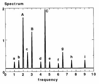
FIG. 6. A schematic spectral analysis of the output from an NN model, where the input were artificial sinusoidal time series of frequencies 2.0, 3.0, and 4.5 (arbitrary units). The three main peaks labeled A, B, and C correspond to the frequencies of the input time series. The nonlinear NN generates extra peaks in the output spec- trum (labeled a–i). The peaks c and g at frequencies of 2.5 and 6.5, respectively, arose from the nonlinear interactions between the main peaks at 2.0 (peak A) and 4.5 (peak C) (as the differ- ence of the frequencies between C and A is 2.5, and the sum of their frequencies is 6.5).
To further simplify the NN models, Tangang et al. (1998b) used EPCAs in- stead of PCAs and a simple pruning method. The spectral analysis method was also introduced to interpret the non- linear interactions in the NN, showing that the nonlinearity of the networks tended to increase with lead time and to become stronger for the eastern regions of the equatorial Pacific Ocean.
THMT compare the correlation skills of NN, CCA, and multiple linear regression (LR) in forecasting the Niño 3 SSTA index. First the PCAs of the tropical Pacific SSTA field and the SLP anomaly field were calculated. The same predictors were chosen for all three methods, namely the first seven SLP anomaly PCA time series at the initial month, and 3 months, 6 months, and 9 months before the initial month (a total of 7 × 4 = 28 predictors); the first 10 SSTA PCA time series at the initial month; and the Niño 3 SSTA at the initial month. These 39 predictors were then further compressed to 12 predictors by an EPCA, and cross-validated model forecasts were made at various lead times after the initial month. Ten CCA modes were used in the CCA model, as fewer CCA modes degraded the forecasts. Figure 8 shows that the NN has better forecast correlation skills than CCA and LR at all lead times, especially at the 12-month lead time (where NN has a correlation skill of 0.54 vs 0.49 for CCA). Figure 9 shows the cross-validated forecasts of the Niño 3 SSTA at 6-month lead time (THMT). In other tropical regions, the advantage of NN over CCA was smaller, and in Niño 4, the CCA slightly outper- formed the NN model. In this comparison, CCA had an advantage over the NN and LR: While the predictand for the NN and LR was Niño 3 SSTA, the predictands for the CCA were actually the first 10 PCA modes of the tropical Pacific SSTA field, from which the regional Niño 3 SSTA was then calculated. Hence during training, the CCA had more information avail- able by using a much broader predictand field than the NN and LR models, which did not have predictand information outside Niño 3.
As the extratropical ENSO variability is much more nonlinear than in the Tropics (Hoerling et al. 1997), it is possible that the performance gap between the nonlinear NN and the linear CCA may widen for forecasts outside the Tropics.
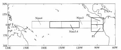
FIG. 7. Regions of interest in the Pacific. SSTA for these regions are used as the predictands in forecast models.
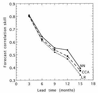
FIG. 8. Forecast correlation skills for the Niño 3 SSTA by the NN, the CCA, and the LR at various lead times (THMT 1998). The cross-validated forecasts were made from the data record (1950–97) by first reserving a small segment of test data, training the models using data not in the segment, then computing fore- cast skills over the test data—with the procedure repeated by shift- ing the segment of test data around the entire record.
8.Nonlinear principal component analysis
PCA is popular because it offers the most efficient linear method for reducing the dimensions of a data- set and extracting the main features. If we are not restricted to using only linear transformations, even more powerful data compression and extraction is generally possible. The NN offers a way to do nonlin- ear PCA (NLPCA) (Kramer 1991; Bishop 1995).
In NLPCA, the NN outputs are the same as the inputs, and data compression is achieved by having relatively few hidden neurons forming a “bottleneck” layer (Fig. 10). Since there are few bottleneck neurons, it would in general not be possible to reproduce the inputs exactly by the output neurons. How many hid- den layers would such an NN require in order to per- form NLPCA? At first, one might think only one hidden layer would be enough. Indeed with one hidden layer and linear activation functions, the NN solution should be identical to the PCA solution. However, even with nonlinear activation functions, the NN solution is still basically that of the linear PCA solution (Bourlard and Kamp 1988). It turns out that for NLPCA, three hidden layers are needed (Fig. 10) (Kramer 1991).
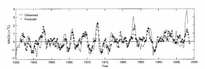
FIG. 9. Forecasts of the Niño 3 SSTA (in °C) at 6-month lead time by an NN model (THMT 1998), with the forecasts indicated by circles and the observations by the solid line. With cross-validation, only the forecasts over the test data are shown here.
The reason is that to properly model nonlinear con The reason is that to properly model nonlinear con- tinuous functions, we need at least one hidden layer between the input layer and the bottleneck layer, and another hidden layer between the bottleneck layer and the output layer (Cybenko 1989). Hence, a nonlinear function maps from the higher-dimension input space to the lower-dimension space represented by the bottleneck layer, and then an inverse transform maps from the bottleneck space back to the original higher- dimensional space represented by the output layer, with the requirement that the output be as close to the input as possible. One approach chooses to have only one neuron in the bottleneck layer, which will extract a single NLPCA mode. To extract higher modes, this first mode is subtracted from the original data, and the pro- cedure is repeated to extract the next NLPCA mode.
Using the NN in Fig. 10, A. H. Monahan (1998, personal communication) extracted the first NLPCA mode for data from the Lorenz (1963) three-component chaotic system. Figure 11 shows the famous Lorenz attractor for a scatterplot of data in the x–z plane. The first PCA mode is simply a horizontal line, explaining 60% of the total variance, while the first NLPCA is the U-shaped curve, explaining 73% of the variance. In general, PCA models data with lines, planes, and hy- perplanes for higher dimensions, while the NLPCA uses curves and curved surfaces.
Malthouse (1998) pointed out a limitation of the Kramer (1991) NLPCA method, with its three hid- den layers. When the curve from the NLPCA crosses itself, for ex- ample forming a circle, the method fails. The reason is that with only one hidden layer between the input and the bottleneck layer, and again one hidden layer between the bottleneck and the output, the non- linear mapping functions are limited to continuous functions (Cybenko 1989), which of course cannot identify 0° with 360°. However, we believe this fail- ure can be corrected by having two hidden layers be- tween the input and bottleneck layers, and two hidden layers between the bottleneck and output layers, since any reasonable function can be modeled with two hid- den layers (Hertz et al. 1991, 142). As the PCA is a cornerstone in modern meteorology–oceanography, a nonlinear generalization of the PCA method by NN is indeed exciting.
9.Neural networks and variational data assimilation
Variational data assimilation (Daley 1991) arose from the need to use data to guide numerical models [including coupled atmosphere–ocean models (Lu and Hsieh 1997, 1998a, 1998b)], whereas neural network models arose from the desire to model the vast em- pirical learning capability of the brain. With such diverse origins, it is no surprise that these two meth- ods have evolved to prominence completely indepen- dently. Yet from section 3, the minimization of the cost function (3) by adjusting the parameters of the NN model is exactly what is done in variational (adjoint) data assimilation, except that here the governing equa- tions are the neural network equations, (1) and (2), instead of the dynamical equations (see appendix for details).
Functionally, as an empirical modeling technique, NN models appear closely related to the familiar lin- ear empirical methods, such as CCA, SVD, PCA, and POP, which belong to the class of singular value or eigenvalue methods. This apparent similarity is some- what misleading, as structurally, the NN model is a variational data assimilation method. An analogy would be the dolphin, which lives in the sea like a fish, but is in fact a highly evolved mammal, hence the natural bond with humans. Similarly, the fact that the NN model is a variational data assimilation method allows it to be bonded naturally to a dynamical model under a variational assimilation formulation. The dy- namical model equations can be placed on equal foot- ing with the NN model equations, with both the dynamical model parameters and initial conditions and the NN parameters found by minimizing a single cost function. This integrated treatment of the empiri- cal and dynamical parts is very different from present forecast systems such as Model Output Statistics (Wilks 1995; Vislocky and Fritsch 1997), where the dynamical model is run first before the statistical method is applied.
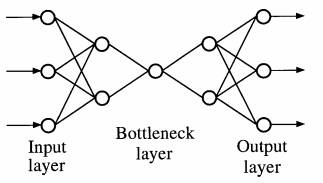
FIG. 10. The NN model for calculating NLPCA. There are three hidden layers between the input layer and the output layer. The middle hidden layer is the “bottleneck” layer. A nonlinear func- tion maps from the higher-dimension input space to the lower- dimension bottleneck space, followed by an inverse transform mapping from the bottleneck space back to the original space rep- resented by the outputs, which are to be as close to the inputs as possible. Data compression is achieved by the bottleneck, with the NLPCA modes described by the bottleneck neurons.
What good would such a union bring? Our present dynamical models have good forecast skills for some variables and poor skills for others (e.g., precipitation, snowfall, ozone concentration, etc.). Yet there may be sufficient data available for these difficult variables that empirical methods such as NN may be useful in improving their forecast skills. Also, hybrid coupled models are already being used for El Niño forecast- ing (Barnett et al. 1993), where a dynamical ocean model is coupled to an empirical atmospheric model. A combined neural–dynamical approach may allow the NN to complement the dynamical model, leading to an improvement of modeling and prediction skills.
10. Conclusions
The introduction of empirical or statistical meth- ods into meteorology and oceanography has been broadly classified as having occurred in four distinct stages: 1) linear regression (and correlation analysis), 2) PCA analysis, 3) CCA (and SVD), and 4) NN. These four stages correspond respectively to the evolv- ing needs of finding 1) a linear relation (or correlation) between two variables x and z; 2) the correlated pat- terns within a set of variables x1 , . . ., xn ; 3) the linear relations between a set of variables x1 , . . ., xn and an- other set of variables z1 , . . ., zm; and 4) the nonlinear relations between x1 , . . ., xn and z1 , . . ., zm. Without ex- ception, in all four stages, the method was first in- vented in a biological–psychological field, long before its adaptation by meteorologists and oceanographers many years or decades later.
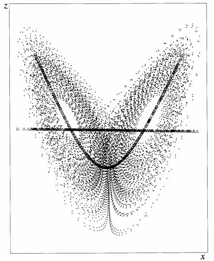
FIG. 11. Data from the Lorenz (1963) three-component (x, y, z) chaotic system were used to perform PCA and NLPCA (using the NN model shown in Fig. 10), with the results displayed as a scatterplot in the x–z plane. The horizontal line is the first PCA mode, while the curve is the first NLPCA mode (A. H. Monahan 1998, personal communication).
Despite the great popularity of the NN models in many fields, there are three obstacles in adapting the NN method to meteorology–oceanography: (a) nonlinear instability, especially with a short data record; (b) overwhelmingly large spatial data fields; and (c) difficulties in interpretting the nonlinear NN results. In large-scale, low-frequency studies, where data records are in general short, the potential success of the unstable nonlinear NN model against stable lin ear models, such as the CCA, de- pends critically on our ability to tame nonlinear instability.
Recent research shows that all three obstacles can be overcome. For obstacle a, ensemble averaging is found to be effective in control- ling nonlinear instability. Penalty and pruning methods and noncon- vergent methods also help. For b, the PCA method is found to be an effective prefilter for greatly reduc- ing the dimension of the large spa- tial data fields. Other possible prefilters include the EPCA, rotated PCA, CCA, and nonlinear PCA by NN models. For c, the mysterious hidden layer can be given a phase space interpretation, and a spectral analysis method aids in understanding the nonlinear NN relations. With these and future im- provements, the nonlinear NN method is evolving to a versatile and powerful technique capable of augmenting traditional linear statis- tical methods in data analysis and in forecasting. The NN model is a type of variational (adjoint) data as- similation, which further allows it to be linked to dynamical models under adjoint data assimilation, potentially leading to a new class of hybrid neural–dynamical models.
References
Badran, F., S. Thiria, and M. Crepon, 1991: Wind ambiguity re- moval by the use of neural network techniques. J. Geophys. Res., 96, 20 521–20 529.
Bankert, R. L., 1994: Cloud classification of AVHRR imagery in maritime regions using a probabilistic neural network. J. Appl. Meteor., 33, 909–918.
Barnett, T. P., and R. Preisendorfer, 1987: Origins and levels of monthly and seasonal forecast skill for United States surface air temperatures determined by canonical correlation analysis. Mon. Wea. Rev., 115, 1825–1850.
Barnston, A. G., and C. F. Ropelewski, 1992: Prediction of ENSO episodes using canonical correlation analysis. J. Climate, 5, 1316–1345.
Bishop, C. M., 1995: Neural Networks for Pattern Recognition. Clarendon Press, 482 pp.
Bourlard, H., and Y. Kamp, 1988: Auto-association by multilayer perceptrons and singular value decomposition. Biol. Cybern., 59, 291–294.
Box, G. P. E., and G. M. Jenkins, 1976: Time Series Analysis: Forecasting and Control. Holden-Day, 575 pp.
Breiman, L., 1996: Bagging predictions. Mach. Learning, 24, 123–140.
Bretherton, C. S., C. Smith, and J. M. Wallace, 1992: An inter- comparison of methods for finding coupled patterns in climate data. J. Climate, 5, 541–560.
Butler, C. T., R. V. Meredith, and A. P. Stogryn, 1996: Retriev- ing atmospheric temperature parameters from dmsp ssm/t-1 data with a neural network. J. Geophys. Res., 101, 7075–7083.
Chauvin, Y., 1990: Generalization performance of overtrained back-propagation networks. Neural Networks. EURASIP Workshop Proceedings, L. B. Almeida and C. J. Wellekens, Eds., Springer-Verlag, 46–55.
Crick, F., 1989: The recent excitement about neural networks. Nature, 337, 129–132
Cybenko, G., 1989: Approximation by superpositions of a sigmoi- dal function. Math. Control, Signals, Syst., 2, 303–314.
Daley, R., 1991: Atmospheric Data Analysis. Cambridge Univer- sity Press, 457 pp.
Derr, V. E., and R. J. Slutz, 1994: Prediction of El Niño events in the Pacific by means of neural networks. AI Applic., 8, 51–63
Elsner, J. B., and A. A. Tsonis, 1992: Nonlinear prediction, chaos, and noise. Bull. Amer. Meteor. Soc., 73, 49–60; Corrigendum, 74, 243.
Finnoff, W., F. Hergert, and H. G. Zimmermann, 1993: Improv- ing model selection by nonconvergent methods. Neural Net- works, 6, 771–783.
French, M. N., W. F. Krajewski, and R. R. Cuykendall, 1992: Rainfall forecasting in space and time using a neural network. J. Hydrol. 137, 1–31.
Galton, F. J., 1885: Regression towards mediocrity in hereditary stature. J. Anthropological Inst., 15, 246–263.
Gately, E., 1995: Neural Networks for Financial Forecasting. Wiley, 169 pp.
Gershenfeld, N. A., and A. S. Weigend, 1994: The future of time series: Learning and understanding. Time Series Prediction: Forecasting the Future and Understanding the Past, A. S. Weigend and N. A. Gershenfeld, Eds., Addison-Wesley, 1–70
Graham, N. E., J. Michaelsen, and T. P. Barnett, 1987: An inves- tigation of the El Niño-Southern Oscillation cycle with statis- tical models, 1, predictor field characteristics. J. Geophys. Res., 92, 14 251–14 270.
Grieger, B., and M. Latif, 1994: Reconstruction of the El Niño Attractor with neural Networks. Climate Dyn., 10, 267–276.
Hastenrath, S., L. Greischar, and J. van Heerden, 1995: Predic- tion of the summer rainfall over south Africa. J. Climate, 8, 1511–1518.
Hertz, J., A. Krogh, and R. G. Palmer, 1991: Introduction to the Theory of Neural Computation, Addison-Wesley, 327 pp.
Hoerling, M. P., A. Kumar, and M. Zhong, 1997: El Nino, La Nina, and the nonlinearity of their teleconnections. J. Climate, 10, 1769–1786.
Hornik, K., M. Stinchcombe, and H. White, 1989: Multilayer feedforward networks are universal approximators. Neural Networks, 2, 359–366.
Hotelling, H., 1936: Relations between two sets of variates. Biometrika, 28, 321–377.
IEEE, 1991: IEEE Conference on Neural Networks for Ocean Engineering. IEEE, 397 pp.
Javidi, B., 1997: Securing information with optical technologies. Physics Today, 50, 27–32.
Kramer, M. A., 1991: Nonlinear principal component analysis using autoassociative neural networks. AIChE J., 37, 233– 243.
Krasnopolsky, V. M., L. C. Breaker, and W. H. Gemmill, 1995: A neural network as a nonlinear transfer function model for retrieving surface wind speeds from the special sensor micro- wave imager. J. Geophys. Res., 100, 11 033–11 045.
Le Cun, Y., J. S. Denker, and S. A. Solla, 1990: Optimal brain damage. Advances in Neural Information Processing Systems II, D. S. Touretzky, Ed., Morgan Kaufmann, 598–605.
Lee, J., R. C. Weger, S. K. Sengupta, and R. M. Welch, 1990: A neural network approach to cloud classification. IEEE Trans. Geosci. Remote Sens., 28, 846–855.
Liu, Q. H., C. Simmer, and E. Ruprecht, 1997: Estimating longwave net radiation at sea surface from the Special Sen- sor Microwave/Imager (SSM/I). J. Appl. Meteor., 36, 919– 930.
Lorenz, E. N., 1956: Empirical orthogonal functions and statisti- cal weather prediction. Statistical Forecasting Project, Dept. of Meteorology, Massachusetts Institute of Technology, Cam- bridge, MA, 49 pp.
Lu, J., and W. W. Hsieh, 1997: Adjoint data assimilation in coupled atmosphere–ocean models: Determining model pa- rameters in a simple equatorial model. Quart. J. Roy. Meteor. Soc., 123, 2115–2139.
Malthouse, E. C., 1998: Limitations of nonlinear PCA as per- formed with generic neural networks. IEEE Trans. Neural Networks, 9, 165–173.
Marzban, C., and G. J. Stumpf, 1996: A neural network for tor- nado prediction based on Doppler radar–derived attributes. J. Appl. Meteor., 35, 617–626.
McCulloch, W. S., and W. Pitts, 1943: A logical calculus of the ideas immanent in neural nets. Bull. Math. Biophys., 5, 115– 137.
Minsky, M., and S. Papert, 1969: Perceptrons. MIT Press, 292 pp. Navone, H. D., and H. A. Ceccatto, 1994: Predicting Indian mon- soon rainfall—A neural network approach. Climate Dyn., 10, 305–312.
Penland, C., 1989: Random forcing and forecasting using principal oscillation pattern analysis. Mon. Wea. Rev., 117, 2165–2185.
Phillips, N. A., 1959: An example of non-linear computational instability. The Atmosphere and the Sea in Motion, Rossby Memorial Volume, Rockefeller Institute Press, 501–504.
Preisendorfer, R. W., 1988: Principal Component Analysis in Meteorology and Oceanography. Elsevier, 425 pp.
Ripley, B. D., 1996: Pattern Recognition and Neural Networks. Cambridge University Press, 403 pp.
Rojas, R., 1996: Neural Networks—A Systematic Introduction. Springer, 502 pp.
Rosenblatt, F., 1962: Principles of Neurodynamics. Spartan, 616 pp.
Rumelhart, D. E., G. E. Hinton, and R. J. Williams, 1986: Learn- ing internal representations by error propagation. Parallel Dis- tributed Processing, D. E. Rumelhart, J. L. McClelland, and P. R. Group, Eds., Vol. 1, MIT Press, 318–362.
Sejnowski, T. J., and C. R. Rosenberg, 1987: Parallel networks that learn to pronounce English text. Complex Syst., 1, 145–168.