GRID SUPERSCALARAND GRICOL: INTEGRATING DIFFERENT PROGRAMMING APPROACHES
Raül Sirvent and Rosa M. Badia
Barcelona Supercomputing Center and UPC, SPAIN
rsirvent@ac.upc.edu
rosab@ac.upc.edu
Natalia Currle-Linde and Michael Resch
High Performance Computing Center Stuttgart (HLRS), University of Stuttgart
linde@hlrs.de
resch@hlrs.de
Abstract
One way to ease the development of Grid applications is to specify and design an Integrated Toolkit which will enable the development of Grid-unaware applications i.e. applications where the Grid is transparent to them but that are able to exploit its resources. Achieving this vision of an Integrated Toolkit requires the investigation and definition of integration between different systems. This paper studies the integration possibilities of GriCoL, a language for the description of complex Grid experiments, andGRIDsuperscalar, a run-time environment which automatically converts sequential program code and deploys it for execution on a Grid. GriCoL operates on a multi-layer paradigm, using both a control flow layer and a data flow layer. We propose integration with GRID superscalar at each of these layers, concluded that integration at the control flowlevel is difficult to achieve but at the data flow level is possible.
Keywords: Grid programming models, Problem solving environments, GRID superscalar, GriCoL.
1. Introduction
The difficulty associated with developing applications to be run on the Grid is a major barrier to adoption of this technology by non-expert users. The challenge in this case is to provide programming environments forGrid-unaware applications, defined as applications where the Grid is transparent to them but that are able to exploit its resources. Furthermore, the challenge is to increase the performance of these applications when possible.
To meet these challenges, one research task of the CoreGRID Institute for Grid Systems, Tools and Environments is the development of an Integrated Toolkit [1]. This task aims to specify and design an Integrated Toolkit which will enable the development of Grid-unaware applications. The run-time of such an integrated toolkit would run these applications in a Grid and optimise their performance dynamically.
The CoreGRID STE vision of an Integrated Toolkit is composed of an Integrated Toolkit run-time and of Integrated Toolkit bindings to different programming languages or to graphical tools and portals. For the specification and design of the Integrated Toolkit, the integration between several different systems is being investigated and defined [1]: ProActive, PadicoTM, GRID superscalar, P-GRADE Portal, Satin/Ibis, GAT/SAGA and the monitoring environment OCM-G. In addition, this paper discusses the integration of GriCoL [2], a language for the description of complex Grid experiments, and GRID superscalar, a run-time environment which automatically converts sequential program code and deploys it for execution on a Grid. Several languages (C/C++, Perl, Java and Shell script) are already supported for programming with GRID superscalar [5].
Figure 1 illustrates a vision of how these various components above can interoperate to realistically build an Integrated Toolkit.
Figure 1. Integrated Toolkit picture
The GriCoL language is Grid-unaware. It is a component-based language for describing complex scientific modeling experiments with a sufficient level of abstraction that the user does not require a knowledge of the Grid or parallel programming. GriCoL is currently utilised within the problem solving environment Science Experimental Grid Laboratory (SEGL)[3], which enables the automated creation, start and monitoring of complex scientific experiments and supports their effective execution on the Grid. SEGL has two main parts: a GUI for the design of the experiment, by working with elements of GriCoL, and a run-time system which chooses the necessary computer resources, organises and controls the sequence of execution according to the task flow and the conditions of the experiment program. Sections 2 and 3 of this paper describe respectively GriCoL and GRID superscalar in more detail and section 4 studies the integration possibilities of these two frameworks as a further step in the realisation of the CoreGRID STE Integrated Toolkit.
2. GriCoL
GriCoL is a universal language for programming complex computer- and data-intensive tasks without being tied to a specific application domain.
GriCoL is a graphical-based language with mixed type and is based on a component-structure model. The main elements of this language are blocks and modules, which have a defined internal structure and interact with each other through a defined set of interfaces.
The language is of an entirely parallel nature. It can implement parallel processing of many data sets at all levels, i.e. inside simple language elements (modules); at the level ofmore complex language structures (blocks) and for the entire experiment. In general, the possibility of parallel execution of operations in all nodes of the experiment program is unlimited.
In order to utilize the capacities of supercomputer applications and to enable interaction with other language elements and structures, it makes use of the principle of wrapping the functionality into components.
Another important property of the language is that it is multi-tiered. This enables the user when describing the experiment to concentrate primarily on the logic of the experiment program and subsequently on the description of the individual parts of the program. The top level of the experiment program is the control flow level, which describes the logical sequence of execution. The main elements of this level are blocks: control blocks and solver blocks. A solver block is the program object which performs some complete operation. The standard example of a solver block can be a simple parameter sweep. The control block is the program object which allows the changing of the sequence of the execution according to a specified criterion. The lower level, the data flow level, provides a detailed description of components at the top level, the control flow level. The main elements of the data flow level are program modules and database sections. The sublayer provides a common description of the database and a section for making additions to the database if necessary. The elements of the language have graphical notation and are represented by icons (for modules and blocks) or as connection lines.
Figure 2 illustrates the abovementioned for anmolecular dynamic simulation at the control flow level.
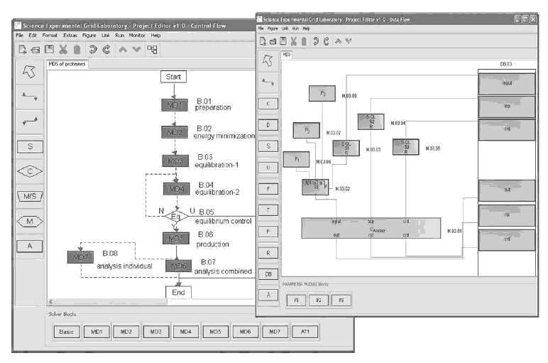
Figure 2. Screenshots of Molecular Dynamics Simulation ((a) Control flow and (b) Data flow of a solver block
As can be seen from this figure the language components make it possible to generate multilayer dynamic-control experiment programs with branches. GriCoL offers the user a complete range of control mechanisms on experiment processes: parallelization, testing of conditions and branching, synchronization and fusion, as well as exchange of messages and signals.
Solver blocks represent the nodes of data processing. Control blocks are either nodes of data analysis or nodes for the synchronization of data computation processes. They evaluate results and then choose a path for further experiment development. Another important language element on the control flow level is the connection line. There are two mechanisms of interaction between blocks which are described with the help of connection lines (either red-solid or bluedashed). If the connection line is blue in colour, the procedure is as follows: each time the computation of an individual data set has been finished, i.e. after completion of a program run within a block, control is transferred to the next block. This process is repeated until all program runs in the block have been completed. That means a pipelined operation on the set of runs. If the connection line is red in colour, control is not passed to the next block before all runs in the previous block have been finished. That means a barrier on the set of runs.
We can illustrate this with an example taken from the field of Molecular Dynamics (MD) simulation, which is a computational method to calculate the time dependent behaviour of a biological molecular system. The left-hand screenshot of figure 2 shows the client visual editor at the control flow level of a large-scale MD simulation study. A total of 3000 different topologies of the system (with different enzyme variants, substrates and starting conditions) are generated in the preparation solver block B.01. The blue-dashed connection lines in figure 2 (e.g. betweenB.01 andB.02) indicate that as soon as a particular simulation task in B.01 has finished, it can be passed on to the next block B.02. A solid line between blocks (e.g. between B.06 and B.07) means that all tasks have to be finished in the preceding block before the control flow proceeds to the next block.
At the data flow level, a typical example of a solver block program is a modeling program (or a program fragment) which cyclically computes a large number of input data sets. At this level, the user can describe the manipulation of data in a very fine grained way. The solver block consists of computation (C), replacement (R), parameterization (P) modules and a database (Exp.DB). These are connected to each other with lines showing the data transfer between modules and the sequence of execution during the computation process. Each module is a Java object, which has a standard structure and consists of several sections. For example: each computation module (C) consists of four sections. The first section organizes the preparation of input data. The second generates the job and controls its execution. The third initializes and controls the record of the result in the experiment data base. The fourth section controls the execution of module operation. It also informs the main program of the block about the manipulation of certain sets of data and when execution within a block is complete. A typical control block program carries out an iterative analysis of the data sets from previous steps of the experiment program and selects either the direction for the further development of the experiment or examines whether the input data sets are ready for further computation, and subsequently synchronizes their further processing.
This example demonstrates an advantage of GriCoL over the many existing tools such as Nimrod[4]or Condor [4]in carrying out complex parameter investigation studies. Nimrod is able to generate parameter sweeps and jobs, running them in a Grid and collecting the data. However, it is unable to perform the task dynamically by generating new parameter sets through an automated optimization strategy. Condor can be used to launch pre-existing parameter studies using distributed resources but gives no special support for dynamic parameter studies.
The right-hand screenshot of figure 2 shows, at the data flow level, the client visual editor for a particular aspect of the previously described MD simulation. It shows the data flowof the equilibration solver block (B.03) fromthe left-hand screenshot (control flow level). The computation module (C-Amber) for the simulation program needs the system topology, the coordinates of the system to start from and an input file. Whereas the system topology and the starting coordinates are taken out of the experiment database via the selection module (S2 and S3), the input files are created for each simulation run individually. Therefore three parameterization modules (P1 -P3) provide the values for the replacement module (R1) that puts these values into an input file skeleton taken from the experiment database (via selection module S1). The resulting output form the simulation is put back into the experiment database.
3. GRID superscalar
As a programming model, GRID superscalar is focused on easing the programming of Grid applications. It is clear that the easiest way of programming for a user is with the desired programming language, in which the user is already an expert, and in a sequential fashion, without using complicated parallel schemes where the user must control syncronizations, message passings, and so on. GRIDsuperscalar achieves this by providing bindings to different programming languages (currently C/C++, Perl, Java and Shell script), and a run-time which automatically executes in parallel the user-defined functions that do not have data dependencies between them. From that source code, GRID superscalar builds internally a workflow with the existing data dependencies between functions, as shown in figure 3, and from that workflow the tasks without dependencies are considered to be run on the Grid. GRID superscalar is not only a programming model, but also a set of tools that allows users to easily gridify an application.
This programming model has been adapted to several environments, currently: Globus (which can work with versions 2 and 4 of the Globus Toolkit [6]), ssh/scp, Ninf-G [7], and the next development version, which adds the data dependence detection between scalar parameters.
In order to program an application with GRID superscalar, a developer must provide amain program, the code of the functions in that specific main program to be executed in the Grid, and an IDL file, which describes the interface of these functions (the type of the parameters, and the direction of these parameters). There is a small set of calls that must be added in the main program:
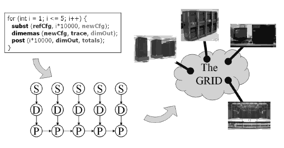
Figure 3. GRID superscalar in a nutshell
GS On for starting the run-time, and GS Off for stopping it. Calls for handling local files (GS Open/GS Close, GS FOpen/GS FClose), as the file is the data unit considered for detecting the dependencies between the functions. Also more advanced, but optional, primitives are provided, such as GS Barrier to wait for all generated tasks to finish, and GS Speculative End to easily create optimization-like algorithms.
GRID superscalar is not only a programming model, but also includes a set of tools in order to ease the porting of the application to the Grid. A tool named Deployment Center allows not only to graphically specify and check the Grid configuration, but also to deploy (send and compile) locally and remotelly the code involved in this developer's project. This deployment step is assisted by gsstubgen, another tool in charge of generating stubs and skeletons needed for allowing the run-time calls, and gsbuilder, responsible for compiling the generated code. This process creates a local client binary and several remote server binaries, which lets a master-worker paradigm application ready to run.
When the user invokes the local binary (the master or client) the run-time comes into action. It starts building a Directed Acyclic Graph containing the data dependencies between the tasks generated till thatmoment, and at the same time starts submitting the tasks which are ready (with no dependencies) to the available machines, thus achieving its parallel execution. In order to decide which is the most suitable host for a task, an estimation of the task's execution time provided by the user is considered, as well as the time that will be spent to transfer all input files required.
The run-time is also in charge of transferring the files needed by a task to the selected host, submitting the task, and after completion, transfer the results back to the master. The input and output files related to a task are kept in the worker till the end of the execution to try to exploit the locality of files, thus saving file transfers. So the results of a task can be used when the task finishes, without having to wait for the transfer to the master to end. When a task has finished, the data dependence graph is updated (this can generate new ready tasks) and the resource becomes available for executing a new task. And at the end of the execution, the remote files are cleaned up, and the remaining results are transferred back to the master, so leaving everything as if it had been a local execution of the application. Other techniques are used in the run-time, such as file renaming to erase false data dependencies, disk sharing to make GRID superscalar aware of data replicas or real shared file systems, checkpointing in order to restart the computation from where it stopped because of a big failure, and ClassAds [8] constraints specification to filter the resources in the Grid. Also dynamic host reconfiguration is offered to add or remove machines to the computation.
For monitoring the execution, the GRID superscalar Monitor can be used. This tool is very useful to visualize the task dependence graph in order to investigate why the application does not reach the desired parallelism. It also shows the status of the tasks: if a task is running it states the machine where the task is running, and when a task is done, it still holds the information about where it has been run, thus providing a graphical way of determining which hosts are executing more tasks.
Regarding the ssh adaptation of the programming model, one of the objectives was to overcome the overhead detected in some Grid middlewares when submitting small granularity jobs. Also if a user wants to work with GRID superscalar inside a cluster it makes no sense in introducing the overhead of calling to a Grid middleware in order to operate between the different nodes, because all the resources are local. Inside a cluster there is no need of encrypted communication, so an easier task notification mechanism can be used, based on TCP/IP sockets.
The Ninf-G adaptation offered several advantages for GRID superscalar when using a Grid middleware. Ninf-G has an advanced file transfer protocol and the possibility of creating persistent workers. Ninf-G is a GridRPC implementation, thus provides a simpler interface, in contrast to Globus, where the job submission is based on building the corresponding RSL.
The current developments of the programming model have a different general approach for achieving the parallelization of the code. Instead of using generation of intermediate code from the IDL file, the new version is based in code annotations and using a source to source compiler. It offers new features such as full support for scalar variables, support for multidimensional arrays and structs only containing scalars, client side worker threads and tracing for post-mortem analysis.
4. Studying the integration possibilities
The first thing to consider when trying to integrate these two tools is their focus. GirCoL is a graphical language, which is based on a component - structure model. The components of GriCoL, e.g. MPI programs or genetic algorithms, are prepared by the programmer by wrapping the code into the component. The user can then create the experiment using these components by using a tool (such as SEGL), which utilizes GriCoL. The program codes are located in the database and during the execution are sent to the currently available resources In the experiment, a database can be used to get input data and store outputs. In contrast, GRID superscalar needs the source code to be provided (the main code and the functions code), and an IDL to describe the interfaces. Then, using the deployment center the code can be automatically sent and compiled in the machines involved in the calculations. This deployment step can be done by the user or by a Grid administrator. Once the deployment has finished, all binaries are available on local and remote machines and then the user can execute himself the main program. Wemust consider also the benefits achieved with the run-time features described in section 3.
Fromthe previous description we can see that each toolmisses what the other tool provides. In particular, the graphical programming language of GriCoL offers a very easy way for non Grid expert users to create experiments, and the database capability also fits into user's needs. In GRID superscalar the deployment features are very suitable for Grid environments, because installing a program in a large set of machines can be a tedious task, and the run-time is also a strong point of the tool, with resource management, checkpointing, and other interesting features.
Looking more deeply into both tools, and considering that GriCoL has two levels ofwork description, we came into two different possibilites of integration:
- Integration at control-flow level.
- Integration at data-flow level.
4.1 Control-flow level integration
In the control-flow integration, GriCoL offers solver blocks and control blocks in order to build the experiment in a higher level vision. So at this level the whole GriCoL experiment (solver blocks and control blocks) can be seen as a GRID superscalar main program where each solver block is a GRID superscalar IDL function, and this main program should describe what the graphical language does (i.e. a translation from graphical to programming language). A solver block can have inside several computing modules (at data-flow level) or even a call to a replacement module (to build a parameter sweep), but this could be seen as different executions inside the same IDL function in the first case, and a call to a more advanced function which performs the parameter sweep in the second.
The main problem we find at this level is that GriCoL only specifies control dependencies, while GRIDsuperscalar is based on data dependencies. The user does not specify at this level the files involved in each solver block, but only the order of these blocks, and conditions or loops to follow with the experiment. Nevertheless, the dependencies between solver blocks could be simulated with dummy files, so GRID superscalar could detect them. By dummy files here we mean files which have nothing to do with the computation, and their only objective is to specify a dependence between two solver blocks.
This can be analysed in more detail. In the case of sequential parts of the experiment, there is no problem for the control of the execution, because GRID superscalar will take into account the dependence generated, and a second solver block will not be executed till the first solver block has finished. So tasks would be generated asynchronously, and a final wait will be performed. The asynchronous task generation scheme also accomplishes the experiment's design in case of solver blocks that can run in parallel.
Although it is possibile to "simulate" the dependencies between different control blocks, the integration at this level will not be natural, because of the different focus of the control-flow level, where data dependencies are not specified. So even being able to generate GRIDsuperscalar tasks, we do not have any information about the files involved in every control block, thus the integration would be very difficult to achieve.
4.2 Data-flow level integration
The second option is an integration at data-flow level, the lowest level from GriCoL. At this level, two different options could be considered:
- Special computing module for a GRID superscalar application.
- Generating tasks froma computing module inside GRIDsuperscalar runtime.
The first possibility willmean a new special type of computing module could be created, and it would be itself a GRID superscalar program. A GriCoL implementation will be responsible for executing the input and output data sections (in charge of transferring the files where needed). This integration will allow final users to build an experiment where some computing blocks use GRID superscalar internally, as it could be done with other special kind of applications (i.e. MPI). The drawback is that GRID superscalar won't have a global view of the computation in the experiment, only inside that computing module, so the benefits from using it would be local. Also a Grid administrator would have to prepare all the different kinds of GRID superscalar applications for making them available to be used from a GriCoL implementation by doing local deployments.
The next option in this data-flowlevel integration is allowing the generation of GRID superscalar tasks from a computing module. Each computing module's functionality could be encapsulated into a GRID superscalar's IDL function, and be called whenever needed. With this approach, a single instance of a GRIDsuperscalar run-time will have a global view of the computation involved in the experiment, as all tasks would be generated for that single run-time. The single run-time could be in charge of resource brokering (submitting the tasks to the corresponding machines), and will provide the rest of the features available in the run-time. Another particularity of this version is that theGriCoL implementation will call to GRID superscalar run-time directly every time a task must be generated. This is particularly suitable for a specific example of a GriCoL solver block, namely one which carries out a simple parameter sweep, because the implementation engine for GriCoL would be responsible for making the calls with the different parameters in this parametric study, so GRID superscalar does not need any extra information to deal with parameter sweep blocks.
4.3 General integrations
From previous discussion we can see that the last option is the most suitable for the objectives of the CoreGRID Task 7.3, that is achieving the creation of an IntegratedToolkit generic enough to handle several programming languages and tools, and making the Grid an invisible layer. There are still other possibilities of integration, but orthogonal to the previous mentioned.
The first one is regarding the code deployment techniques used in GRID superscalar. It is clear that integrating these techniques in the final solution would be very useful for a Grid administrator in order to install the services needed in the machines related to the experiment. Every code or simulator implemented as a solver block could be wrapped into a GRID superscalar IDL function, and then could be easily deployed as it is done in GRID superscalar.
And the second orthogonal integration is about the database support provided inGriCoL. The data unit forGRIDsuperscalar is the file, whileGriCoL supports defining interaction with a database in order to get or store the data needed for the experiment. This feature is important, as scientific data is usually stored in databases. So, GRID superscalar must be aware of those databases, and use them as a way to treat data from the different experiments instead of working only with files.
5. Conclusions and future work
With the proposed integration of these two tools, we achieve a unique solution for several ways of programming the Grid. The first one is GriCoL, focused on graphical design of experiments, and the second is programming from source code, as can be done with GRID superscalar. This paper presents an initial solution for the integration, and establishes a basic step towards the creation of the Integrated Toolkit described in CoreGRID Task 7.3, by simplifying the development of Grid applications and allowing the execution of applications in the Grid in a transparent way.
Regarding future work, a deeper study for integrating the database support in the final solution should be performed. Also the integration of the message passing features specified in GriCoL could be considered.
Acknowledgments
Thiswork has been partially supported byNoECoreGRID(FP6-004265) and by the Ministry of Science and Technology of Spain under contract TIN2004- 07739-C02-01.
References
- CoreGRID Institute for Grid Systems, Tools and EnvironmentsRoadmap version 2 on Grid Systems, Tools and Environments. CoreGRID deliverable D.STE.04, 2006.
- N. Currle-Linde and M. Resch. Gricol: A Language for Grid Computing. In Grid2006, Barcelona, Spain, 2006. To appear.
- N. Currle-Linde, U. Kuester, M. Resch, and B. Risio. Science experimental grid laboratory (segl) dynamical parameter study in distributed systems. In ParCo 2005 - Parallel Computing, Malaga, Spain, September 2005.
- A. de Vivo, M. Yarrow, K. McCann. A comparison of parameter study creation and job submission tools. In Technical report NAS-01002, NASA Ames Research Center, Moffet Filed, CA, 2000.
- R.M. Badia, J. Labarta, R. Sirvent, J.M. P´erez, J.M. Cela, R. Grima. Programming Grid Applications with GRID Superscalar. Journal of Grid Computing, 1(2):151-170, 2003.
- I. Foster, C. Kesselman. Globus: A Metacomputing Infrastructure Toolkit. Int. Journal of Supercomputer Applications, 11(2):115-12
- Y. Tanaka, H. Nakada, S. Sekiguchi, T. Suzumura, S. Matsuoka. Ninf-G: A Reference Implementation of RPC-based Programming Middleware for Grid Computing. Journal of Grid Computing, 1(1):41-51, 2003.
- R. Raman, M. Livny, M. Solomon. Matchmaking: Distributed Resource Management for High Throughput Computing. Proceedings of the Seventh IEEE International Symposium on High Performance Distributed Computing, July 28-31, 1998, Chicago, IL.