SEGL: A Problem Solving Environment for the Design and Execution of Complex Scientific Grid Applications
N. Currle-Linde, M. Resch and U. Küster
High Performance Computing Center Stuttgart (HLRS), University of Stuttgart,
Nobelstraße 19, 70569 Stuttgart, Germany
linde@hlrs.de
resch@hlrs.de
kuester@ac.upc.edu
Abstract
The design and execution of complex scientific applications in the Grid is a difficult and work-intensive process which can be simplified and optimized by the use of an appropriate tool for the creation and management of the experiment. We propose SEGL (Science Experimental Grid Laboratory) as a problem solving environment for the optimized design and execution of complex scientific Grid applications. SEGL utilizes GriCoL (Grid Concurrent Language), a simple and efficient language for the description of complex Grid experiments.
1 Introduction
The development of Grid technology [1] provides the technical possibilities for a comprehensive analysis of big data volume for practically all application environments. As a consequence, scientists and engineer are producing an increasing number of complex applications which make use of distributed Grid resources. However, the existing Grid services do not allow scientists to design complex applications on a high level of organization [2]. For this purpose they require an integrated interface which makes it possible to automate the creation and starting as well as the monitoring of complex experiments and to support their execution with the help of the existing resources. This interface must be designed in such a way that it does not require the user to have a knowledge of the Grid structure or of a programming language. In this paper, we propose SEGL (Science Experimental Grid Laboratory) as a problem solving environment for the design and execution of complex scientific Grid applications. SEGL utilizes GriCoL (Grid Concurrent Language) [3], a simple and efficient language for the description of complex Grid experiments.
1.1 Existing Tools for Parameter Investigation Studies
There are some efforts in implementing such tools e.g. Nimrod [4], Ilab [4]. These tools are able to generate parameter sweeps and jobs, running them in a distributed computer environment (Grid) and collecting the data. ILab also allows the calculation of multi-parametric models in independent separate tasks in a complicated workflow for multiple stages. However, none of these tools is able to perform the task dynamically by generating new parameter sets by an automated optimization strategy as is needed for handling complex parameter problems.
1.2 Dynamic Parameterization
Complex parameter studies can be facilitated by allowing the system to dynamically select parameter sets on the basis of previous intermediate results. This dynamic parameterization capability requires an iterative, self-steering approach. Possible strategies for the dynamic selection of parameter sets include genetic algorithms, gradient-based searches in the parameter space, and linear and nonlinear optimization techniques. An effective tool requires support of the creation of applications of any degree of complexity, including unlimited levels of parameterization, iterative processing, data archiving, logical branching, and the synchronization of parallel branches and processes. The parameterization of data is an extremely difficult and time-consuming process. Moreover, users are very sensitive to the level of automation during application preparation. They must be able to define a fine-grained logical execution process, to identify the position in the input data of parameters to be changed during the course of the experiment, as well as to formulate parameterization rules. Other details of the parameter study generation are best hidden from the user.
SEGL (Science Experimental Grid Laboratory) aims to overcome the above limitations of existing systems. The new technology has a sufficient level of abstraction to enable a user, without knowledge of the Grid or parallel programming, to efficiently create complex modeling experiments and execute them with the maximum efficient use of the Grid resources available.
This paper is organized as follows: In the third section we describe properties and principle of organization of an parallel language GriCoL for the description of Grid experiments. The fourth section presents the architecture of SEGL, namely the Experiment Designer and the Runtime System.
2 Science Experimental Grid Laboratory (SEGL)
Science Experimental Grid Laboratory (SEGL) is a problem solving environment enabling the automated creation, start and monitoring of complex experiments and supports its effective execution on the Grid. Figure 1 shows the system architecture of SEGL at a conceptual level. It consists of three main components: the UserWorkstation (Client), the ApplicationServer (Server) and the ExpDBServer (OODB). The system operates according to a Client-Server-Model in which the ApplicationServer interacts with remote target computers using a Grid Middleware [6,7]. The implementation is based on the Java 2 Platform Enterprise Edition (J2EE) specification and JBOSS Application Server. The database used is an Object Oriented Database (OODB) with a library tailored to the application domain of the experiment.
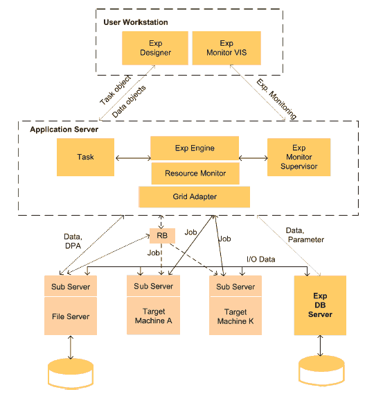
Fig. 1. Conceptual Architecture of SEGL
The two key parts of SEGL are: Experiment Designer (ExpDesigner), used for the design of experiments by working with elements of GriCoL, and the runtime system (ExpEngine).
3 Grid Concurrent Language
From the user's perspective, complex experiment scenarios are realized in Experiment Designer using GriCoL to represent the experiment.
GriCoL is a graphical-based language with mixed type and is based on a component model. The main elements of this language are components, which have a defined internal structure and interact with each other through a defined set of interfaces. In addition, language components can have structured dialog windows through which additional operators can be written into these elements.
The language is of an entirely parallel nature. GriCoL provides parallel processing of many data sets at all levels, i.e. inside simple language components; at the level of more complex language structures and for the entire experiment. In general, the possibility of parallel execution of operations in all nodes of the experiment program is unlimited.
The language is based on the principle of wrapping functionality in components in order to utilize the capacities of supercomputer applications and to enable interaction with other language elements and structures. Program codes, which may be generated in any language, for parallel machines are wrapped in the standard language capsule.
Another property of the language is its extensibility. The language enables new functional components to be added to the language library.
An additional property of the language is that it is multi-tiered. The multitiered model of organization enables the user when describing the experiment to concentrate primarily on the common logic of the experiment program and subsequently on the description of the individual fragments of the program.
GriCoL has a two-layer model for the description of the experiment and an additional sub-layer for the description of the repository of the experiment. The top level of the experiment program, the control flow level is intended for the description of the logical stages of the experiment. The main elements of this level are blocks and connection lines. The lower level, the data flow level, provides a detailed description of components at the top level. The main elements of the data flow level are program modules and database areas. The repository sublayer provides a common description of the database.
3.1 Control Flow Level
To describe the logic of the experiment, the control flow level offers different types of blocks: solver blocks, condition blocks, merge/synchro blocks and message blocks. Solver blocks represent the nodes of data processing. Control blocks are either nodes of data analysis or nodes for the synchronization of data computation processes. They evaluate results and then choose a path for further experiment development.
Another important language element on the control flow level is the connection line. Connection lines indicate the sequence of execution of blocks in the experiment. There are two mechanisms of interaction between blocks. If the connection line is red (solid) in color, control is passed to the next block one time only i.e. after all runs in the previous block have been finished. If the connection line is blue (dashed) in color, control is transferred to the next block many times i.e. after each computation of an individual data set has been completed. In accordance with the color of the input and output lines, the blocks interact with each other in two modes: batch and pipeline.
Figure 2(a) shows an example of an experiment program at the control flow level. The start block begins a parallel operation in solver blocks B.01 and B.02. After execution of B.02, processes begin in solver blocks B.03 and B.04. Each data set which has been computed in B.04 is evaluated in control block B.05. The data sets meeting the criterion are selected for further computation. These operations are repeated until all data sets from the output of B.04 have been evaluated. The data sets selected in this way are synchronized by a merge/synchro block with the corresponding data sets of the other inputs of B.06. The final computation takes place in solver block B.07.
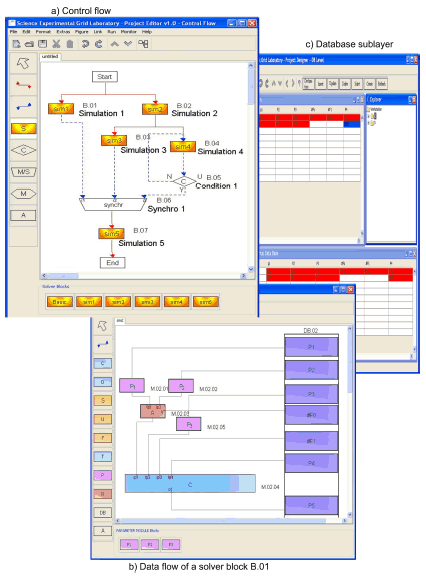
Fig. 2. Experiment Program
3.2 Data Flow Level
A detail of programming on the data flow level is represented on Figure 2(b). The solver block consists of computation (C), replacement (R), parameterization (P) modules and a database (DB). Computation modules are functional programs which organize and execute data processing on the Grid resources. The programs of computation modules consists of two parts: the resident program, which is executed on the application server, and the remote program, which is executed on the Grid resources. Some computation modules have one resident program but can have several remote programs, if the executable code of the programs of the remote computers differ from each other. On one hand, the resident program supports the interaction with other language modules and, on the other hand, starts the copies of its remote programs on the target machines. In addition it organizes the preparation of input data sets for the computation and writes the results into the experiment database. Parameterization modules are modules which generate parameter values. Replacement modules are modules for remote parameterizations. A more detailed description of the working of the solver modules is given in [3].
Figure 2(b) shows an example of a solver block program. A typical example of a solver block program is a modeling program which cyclically computes a large number of input data sets. In this example three variants of parameterization are represented:
(a) Direct transmission of the parameter values with the job (Parameter 3);
(b) Parameterized objects are large arrays of information (Parameter 4) which are kept in the experiment database;
(c) Parameters of jobs are large arrays of information which are modified by replacement module (M.02.03) for each run with new values generated by parameter modules (M.02.01 and M.02.02).
A more detailed description can be found in [3].
4 Science Experimental Grid Laboratory Architecture
Figure 3 shows the architecture of the Experiment Designer. The Experiment Designer contains several components for the design of the experiment program: ProgramConstructor, TaskGenerator, DBConstructor, DBBrowser and MonitorVisGenerator. To add new functional modules to the language library the component Units Library Assistant is used.
The key component of the Experiment Designer is the Program Constructor. Within this environment, the user creates a graphical description of the experiment on three levels: the control flow, data flow and the repository layers.
After the completion of the graphical description of an experiment, the user reviews the execution of the experiment with the aim of verifying the logic of the experiment and also detecting inaccuracies in programming.
After completion of the design of the program at the graphical icon-level, it is compiled. During the compiling the following is created:
(a) The program objects (modules), which belong to the block are incorporated in Block Containers;
(b) Block Containers are incorporated in the Task Container.
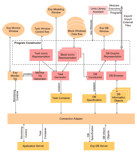
Fig. 3. Architecture of Experiment Designer
In addition, the Task Container also includes the Block Connection @ Activity Table. This table describes the sequence of execution of experiment program blocks. At the control flow level, when a new connection is made between the output of a block and the input of the next block, a new element is created in the Block Connection @ Activity Table to describe the connection.
Parallel to this, the DBConstructor aggregates the arrays of data icon-objects from all blocks and generates QL-descriptions of the experiment's database (DBSpecification). The Task Container is transferred to the Application Server and the QL-descriptions are transferred to the experiment database server. In addition the Experiment Designer has a DBBrowser; its function is to convert the files and program modules into the object form (DBInformationObjects) required for writing to the database. Besides, the DBBrowser makes it possible to observe the current state of the experiment database as well as to read and write information objects. Additionally, Experiment Designer has the MonitorVisGenerator. This program creates the windows for the control and monitoring of the experiment.
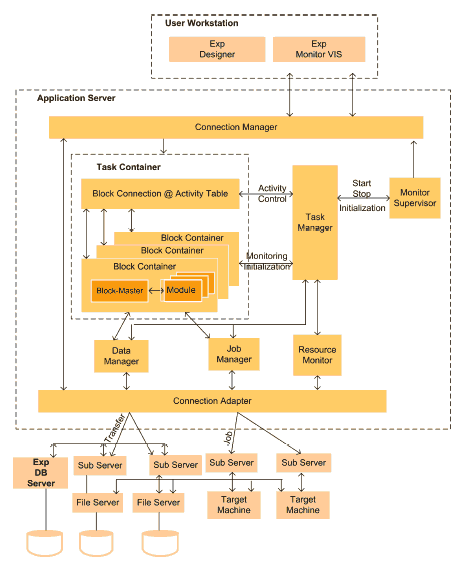
Fig. 4. Conceptual Architecture of SEGL
4.1 Runtime System
The runtime system of SEGL (ExpEngine) chooses the necessary computer resources, organizes and controls the sequence of execution according to the task flow and the condition of the experiment program, monitors and steers the experiment, informing the user of the current status (see Figure 4). This is described in more detail below.
The Application Server consists of the ExpEngine, Task, the MonitorSupervisor and the ResourceMonitor. The Task is the container application (Task Container). The ResourceMonitor holds information about the available resources in the Grid environment. The MonitorSupervisor controls the work of the runtime system and informs the Client about the current status of the jobs and the individual processes. The ExpEngine is the controlling subsystem of SEGL (runtime subsystem). It consists of three subsystems: the TaskManager, the JobManager and the DataManager. The TaskManager is the central dispatcher of the ExpEngine. It coordinates the work of the DataManager and the JobManager.
- It organizes and controls the sequence of execution of the program blocks. It starts the execution of the program blocks according to the task flow and the condition of experiment program.
- It activates a particular block according to the task flow, chooses the necessary computer resources for the execution of the program and deactivates the block when this section of the program has been executed.
It informs the MonitorSupervisor about the current status of the program.
The DataManager organizes data exchange between the ApplicationServer and the FileServer and between the FileServer and the ExpDBServer. Furthermore, it controls all parameterization processes of input data. The JobManager generates jobs, places them in the corresponding SubServer of the target machines. It controls the placing of jobs in the queue and observes their execution. The SubServer informs the JobManager about the status of the execution of the jobs.
The final component of the SEGL is the database server (ExpDBServer). All data which occurred during the experiment, initial and generated, are kept in the ExpDBServer. The ExpDBServer also hosts a library tailored to the application domain of the experiment. For the realization of the database we choose an object-oriented database because its functional capabilities meet the requirements of an information repository for scientific experiments. The interaction between ApplicationServer and the Grid resources is done through a Grid adaptor.
4.2 Block Connection @ Activity Table
The Block Connection @ Activity Table (BC@AT) contains information about the conditions and the sequence between individual experiment blocks. Whenever a block is activated (i.e. a connection made between the output of a block and the input of another block), an entry in this table is made. The table is shown in Figure 5. Each element of the table consists of two parts. The left part relates to the exit of the block while the right part is concerned with the input of the block.
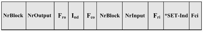
Fig. 5. Block Connection @ Activity Table
- The left part of the BC@AT has the following elements:
NrBlock - Block number (identifier).
NrOutput - Number of the block exit.
Fro - Activation flag of the run. Fro is a counter. After the run has been
finished, the value of Fro becomes 1. After the transfer of the activation
signal from the left side to the right side, the value of Fri becomes 1 and the
value of Fro becomes 0.
Ind - Index of the run currently being executed.
Fco - When set to "1" means the completion of the operation running. - The right part of the BC@AT has the following elements:
NrBlock - Block number (identifier).
NrInput - Number of the block input.
Fri - Activation flag of the input data set. The right block sets the value
of the counter to 1 as soon as the computation of the following data set
is started. This value of the flag is zero when the input has not yet been
activated.
*SET-Ind - Index of the data sets. *SET-Ind contains the reference to the
buffer, into which the TaskManager writes the indices of the input data
which are ready for computation.
Fci - Activation flag for all sets of input data. It also signals complete processing
when set to "1".
Figure 6 shows an example of the connection table BC@AT for the experiment at the control flow level shown in Figure 2(a).
The main program of the block is the master program, which controls the execution of inter-block operations. After the processing of one of the data sets has been finished or the computation of all sets of input data has been terminated, these events are registered in the BC@AT with a special flag. In this way, the partial or complete execution of block operations is signalized. After the execution of all programs in the block has been finished, the Fco flag signifying the termination of all block operations is set. Depending on the logic of the experiment, the user will himself decide whether to use the Fro flag or not. (The Fro flag is used in the case of pipelined operations: blue-dashed line.) The design of each block already provides the possibility to set such a flag after the execution of a run. In this case each time the execution of a run in the previous block has been finished the corresponding operations in the following block can be started.
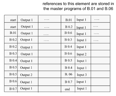
Fig. 6. BC@AT for Figure 2
After the experiment has been started the TaskManager cyclically scans the state of the activation flags belonging to the block exits (see left part of the table). When an activation flag has been found, the TaskManager activates the corresponding activation flag of the entrance of the following block (right part of the table). Immediately after the blocks have been started their master programs cyclically ask for the state of the corresponding input flags. As soon as the activation flag has been placed in the connection table BC@AT (relating to the entrances of blocks), the master program receives a corresponding message together with the number of the run carried out by the previous block. The number stands for a run which has already been finished and for the corresponding run of the following block which is now ready for computation. Once the input data set has been prepared the master program initiates the computation of the corresponding data in the block.
5 Use Case: Molecular Dynamics Simulation of Proteins
Molecular Dynamics (MD) simulation is one of the principal tools in the theoretical study of biological molecules. This computational method calculates the time dependent behavior of a molecular system. MD simulations have provided detailed information on the fluctuations and conformational changes of proteins and nucleic acids. These methods are now routinely used to investigate the structure, dynamics and thermodynamics of biological molecules and their interaction with substrates, ligands, and inhibitors.
A common task for a computational biologist is to investigate the determinants of substrate specificity of an enzyme. On one hand, the same naturally occurring enzyme converts some substrates better than others. One the other hand, often mutations are found, in nature or by laboratory experiments, which change the substrate specificity, sometimes in a dramatic way. To understand these effects, multiple MD simulations are performed consisting of different enzyme-substrate combinations. The ultimate goal is to establish a general, generic molecular model that describes the substrate specificity of an enzyme and predicts short- and long-range effects of mutations on structure, dynamics, and biochemical properties of the protein.
While most projects on MD simulation are still managed by hand, large-scale MD simulation studies may involve up to thousands of MD simulations. Each simulation will typically produce a trajectory output file with a size of several gigabytes, so that data storage, management and analysis become a serious challenge. These tasks can no longer be performed by batch jobs and therefore have to be automated. Therefore it is worthwhile to use an experiment management system that provides a language (GriCoL) that is able to describe all the necessary functionalities to design complex MD parameter studies. The experiment management system must be combined with the control of job execution in a distributed computing environment. Figure 6 shows the schematic setup of a large-scale MD simulation study. Starting from user provided structures of the enzyme, enzyme variants (a total of 30) and substrates (a total of 10), in the first step the preparation solver block (B.01) is used to generate all possible enzyme substrate combinations (a total of 300). This is accomplished by using the select module in the data flow of the preparation solver block, which builds the Cartesian product of all enzyme variants and substrates. Afterwards for all combinations the molecular system topology is built. These topologies describe the system under investigation for the MD simulation program. All 300 topology files are stored in the experiment database and serve as an input for the equilibration solver block (B.02). For better statistical analysis and sampling of the proteins' conformational space, each system must be simulated 10 times, using a different starting condition each time. Here the replacement and parameterization modules of the GriCoL language are used in the data flow of the equilibration solver block to generate automatically all the necessary input files and job descriptions for the 3,000 simulations. The equilibration solver block now starts an equilibration run for each of the 3,000 systems, which usually needs days to weeks, strongly depending on the numbers of CPUs available and the size of the system. In the equilibration run the system should reach equilibrium. An automatic control of the system's relaxation into equilibrium would be of great interest to save calculation time. This can be achieved by monitoring multiple system properties at frequent intervals. The equilibrium control block (B.03) is used for this. Once the conditions for equilibrium are met, the equilibration phase for this system will be terminated and the production solver block (B.04) is started for this particular system. Systems that have not reached the equilibrium yet are subjected to another round of the equilibration solver block (B.02). During the production solver block (B.04), which performs a MD simulation with a predefined amount of simulation steps, equilibrium properties of the system are assembled. Afterwards the trajectories from the production run are subjected to different analysis tools. While some analysis tools are run for each individual trajectory (B.05), some tools need all trajectories for their analysis (B.06). The connection line between B.01 and B.02, as well as between B.04, B.06 and the end block of the control flow is drawn in red-solid, because in these blocks all tasks have to be finished before the control flow proceeds to the next block. The blue-dashed lines used to connect the other blocks indicate that as soon as one of the simulation tasks has finished, it can be passed to the next block. This example shows the ability of the simple control flow to steer the laborious process of a large number of single tasks in an intuitive way. The benefits of using an experiment management system like this are obvious. Beside the time saved for setting up, submitting, and monitoring the thousands of jobs, the base for common errors like misspelling in input files is also minimized. The equilibration control helps to minimize simulation overhead as simulations which have already reached equilibrium are submitted to the production phase while others that have not are simulated further. The storage of simulation results in the experiment database enables the scientist to later retrieve and compare the results easily.
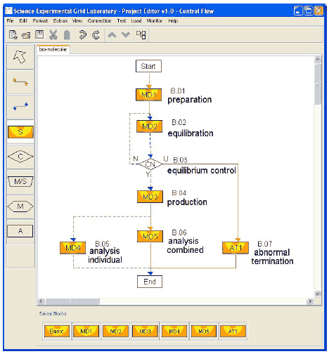
Fig. 7. Screenshot of bio-molecular experiment
6 Conclusion
This paper presented a powerful integrated system for the creation, execution and monitoring of complex modeling experiments in the Grid. The integrated system is composed of GriCoL, a universal abstract language for the description of Grid experiments and SEGL, a problem solving environment capable of utilizing the resources of the Grid to execute and manage complex scientific Grid applications. The new technology has a sufficient level of abstraction to enable a user, without knowledge of the Grid or parallel programming, to efficiently create complex modeling experiments and execute them with the maximum efficient use of the Grid resources available.
Acknowledgment
This research work is carried out under the FP6 Network of Excellence Core- GRID funded by the European Commission (Contract IST-2002-004265).
References
- Foster, I., Kesselman, C.: The Grid: blueprint for a future computing infrastructure. Morgan Kaufmann Publishers, USA (1999)
- Yarrow, M., McCann, K., Biswas, R., van der Wijngaart, R.: An advanced user interface approach for complex parameter study process specification on the information power Grid. In: Proc. of theWorkshop on Grid Computing, Bangalore, India (2002)
- Currle-Linde, N., B¨os, F., Resch, M.: GriCoL: A language for Scientific Grids. In: Sloot, P., van Albada, G., Bubak, M., Trefethen, A. (eds.) Proc. of the 2nd IEEE International Conference on e-Science and Grid Computing, Amsterdam, p. 62 (2006)
- De Vivo, A., Yarrow, M., McCann, K.: A comparison of parameter study creation and job submission tools. Technical report NAS-01002, NASA Ames Research Center, Moffet Filed, CA (2000)
- Yu, J., Buyya, R.: J. Grid Comput. 3(3-4), 171–200 (2005)
- Erwin, D.: Joint project report for the BMBF Project UNICORE Plus, Grant Number: 01 IR 001 A-D (2002)
- Foster, I., Kesselman, C.: J. Supercomputer Appl. 11(2), 115–128 (1997)