
Source of information: http://citeseerx.ist.psu.edu/viewdoc/download?doi=10.1.1.99.2531&rep=rep1&type=pdf
A system architecture and method for tracking people is presented for a sports application. The system input is video data from static cameras with overlapping fields-of-view at a football stadium. The output is the real-world, real-time positions of football players for during a match. The system comprises two processing stages, operating on data from first a single camera and then multiple cameras. The organisation of processing is designed to achieve sufficient synchronisation between cameras, using a request-response pattern, invoked by the second stage multi-camera tracker. The single-view processing includes change detection against an adaptive background and image-plane tracking to improve the reliability of measurements of occluded players. The multi-view process uses Kalman trackers to model the player position and velocity, to which the multiple measurements input from the single-view stage are associated. Results are demonstrated on real data.
This paper presents an architecture, and method, to allow multiple people to be tracked with multiple cameras. The application output is the positions of players, and ball, during a football match. This output can be used for entertainment – augmenting digital TV, or low-bandwidth match play animations for web or wireless display; and also for analysis of fitness and tactics of the teams and players.
Several research projects on tracking soccer players have published results. Intille and Bobick [4] track players, using the concept of closed-world, in the broadcast TV footage of American football games. A monocular TV sequence is also the input data for [6], in which panoramic views and player trajectories are computed. The SoccerMan [1] project analyses two synchronised video sequences of a soccer game and generates an animated virtual 3D view of the given scene. Similarly to TV data, these projects use one (or two) pan-tilt- zoom camera to improve the image resolution of players, and the correspondence between frames has to be made on the basis of matching field lines or arcs. An alternative approach to improving players' resolution is to use multiple stationary cameras. Although this method requires dedicated static cameras, it increases the overall field of view, minimizes the effects of dynamic occlusion, provides 3D estimates of ball location, and improves the accuracy and robustness of estimation due to information fusion. There are different ways to use multi-view data, e.g. hand-off between best-view cameras, homography transform between the images of uncalibrated cameras, or using calibrated cameras able to determine the 3D world coordinate with the cooperation of two or more cameras.
Our system uses eight digital video cameras statically positioned around the stadium, and calibrated to a common ground-plane co-ordinate system using Tsai's algorithm. A two-stage processing architecture is used. Details of this architecture are provided in Section 2. The first processing stage is the extraction of information from the image streams about the players observed by each camera. This is described in Section 3. The data from each camera is input to a central tracking process, described in Section 4, to update the state estimates of the players. This includes the estimate of which of the five possible uniforms each player is wearing (two outfield teams, two goal-keepers, and the three referees. In this paper, ‘player’ includes the referees). The output from this central tracking process is the 25 player positions per time step. The tracker indicates the category (team) of each player, and maintains the correct number of players in each category. The identification of individual players is not possible, given the resolution of input data, so only team is recognised. The ball tracking methods are outside the scope of this paper.
In the video processing stage, a three step approach is used to generate the Features. Each Feature consists of a 2D ground- plane position, its spatial covariance, and a category estimate. Every camera will be connected to a processing unit called a ‘Feature Server’, reflecting its position in the overall architecture.
Features are collected and synchronised by the centralised ‘Tracker’ and are duly processed to generate a single model of the game (state) at a given time. This game-state is finally passed through a phase of marking-up which will be responsible for generating the XML output that is used by third party applications to deliver results to their respective target audiences.
The cameras are positioned at relevant locations around the stadium and are connected to a series of eight ‘Feature Servers’ through a network of fibre optics, see Fig 1. The position of the cameras is governed by the layout of the chosen stadium and the requirement to achieve an optimal view of the football pitch (Good resolution of each area, especially the goal-mouths, is more important than multiple views of each area).
Each optical fibre terminates in a location which houses all of the processing hardware (eight Feature Servers and a single Tracker) where the digital video is interpreted into useable image streams. The ‘Feature Servers’ are interconnected with the ‘Tracker’ hardware using an IP/Ethernet network which is used to communicate and synchronise the generated Features. This configuration of physical location of components is influenced by the requirement to minimise the profile of the installations above the stadium. If that requirement were not so important, the overall bandwidth requirements could be considerably reduced by locating the Feature Servers alongside the cameras. Then, only the Features would need transporting along the long distance to the ‘Tracker’ processing stage: this could be achieved with regular or even wireless Ethernet, rather than the optic fibre presently needed.
A ‘request-response’ mechanism is selected to communicate the Features from the Feature Servers to the Tracker. This solves several of the problems inherent with managing eight simultaneous streams of data across a network.
The Tracker is responsible for orchestrating the process by which Feature Servers generate their Features. Each iteration (frame) of the process takes the form of a single (broadcast) request issued by the Tracker at a given time. The Feature Servers then respond by taking the latest frame in the video stream, processing it and transmitting the resultant Features back to the Tracker. Synchronisation of the Features is implied as the Tracker will record the time at which the request was made.
The Request-Response action repeats continually while the time-stamped Features are passed on to be processed by components running in parallel inside of the Tracker. The results of the Tracking components are then marked up (into XML) and delivered through a peer-to-peer connection with any compliant third party application.
The second stage (‘Tracker’) process does not have access to video data processed in the first stage. Therefore, the ‘Feature’ data must include all that is required by the second stage components to generate reliable estimates position for the people (and ball) present on the football pitch. The composition of the Feature is thus dictated by the requirements of the second stage process. The process described in section 4 requires the bounding box, estimated ground-plane location and covariance, and the category estimate (defined as a seven-element vector, the elements summing to one, and corresponding to the five different uniforms, the ball, and ‘other’). Further information is included, e.g. the single-view tracker ID tag, so that the multi- view tracker can implement track-to-track data association [2]. Common software development design patterns are used to manage the process of transmitting these Features to the ‘Tracker’ hardware by managing the process of serialising to and from a byte stream (UDP Socket). This includes the task of ensuring compatibility between different platforms.
Each of the many software components requires a degree of configuration, whether it is a simple instruction or a complex data file (e.g. Camera to ground calibration). Coupled with the combination of eight Feature Servers, eight Cameras and a single Tracker this process will be difficult for the individual. Therefore, a centrally managed system is necessary.
A message based network protocol has been devised to control and configure the operations of the various components. This protocol will also provide support for other operations, such as image retrieval for camera calibration.
The Feature Server uses a three step approach is used to generate the Features, as indicated in Fig. 1. Each Feature consists of a 2D ground-plane position, its spatial covariance, and a category estimate.
The first step is ‘Change Detection’ based on image differencing: its output is connected foreground regions (Fig. 2, top). An initial background is modelled using a mixture of Gaussians and learned beforehand. The initial background is then used by the running average algorithm for fast updating. If Fk is the foreground binary map at time k, then the background is updated with image y as:
μ k = [αL y + (1 - α L) μ k-1 ]Fk + [ α H y + (1 - αH)μk-1]Fk
where 0 < αL << α H << 1 .
The second step is a local tracking process [8] to split Features of grouped people. The bounding box and centroid co-ordinates of each player are used as state and measurement variables in a Kalman filter:
x = [rc cc rc cc Δr1 Δc1 Δr2 Δc2 ]T
z = [rc cc r1 c1 r2 c2 ]T
where (rc, cc) is the centroid, r1, c1, r2, c2 represent the top, left, bottom and right bounding edges, respectively. (Δr1 Δc1 ) and (Δr2 Δc2 ) are the relative positions of the bounding box corners to the centroid.

As in [8], it is assumed that each target has a slowly varying height and width. Once some bounding edge of a target is decided to be observable, its opposite, unobservable bounding edge can be roughly estimated (Fig. 2). Because the estimate is updated using partial measurements whenever available, it is more accurate than using prediction only.
For an isolated player, the image measurement comes from foreground region directly, which prevents estimation errors accumulating from a hierarchy of Kalman filters. We assume measurement covariance is constant because foreground detection is a pixelwise operation:
u = [r2 cc ]T
Λu = Λ0
For a grouped player, the measurement is calculated from the estimate and the covariance increases to Λ u = βΛ 0 ( β > 1 ).
Writing the homography transform from i-th image plane to ground plane as H i , and the ground plane measurement as
zi = [X w Yw ]T , the homogeneous coordinates for the ground plane and i-th image plane can be written as X = [ (z i ) T W ]T , x = [uT 1]T respectively, and X = Hix
The measurement covariance in the ground plane in homogeneous coordinates is [3]:
ΛX = BΛ h BT + HΛx HT
where B is the matrix form of ~ , h is the vector form of H, with covariance Λh , Λis the conversion of Λ u to homogeneous coordinates. While the second item is the propagation of image measurement errors, the first item explains the errors in the homography matrix, which depends on the accuracy, number and distribution of the landmark points used to compute the matrix. The conversion of Λ X to inhomogeneous coordinates is the ground plane covariance Ri . Fig. 4 shows the ground plane measurement covariance.

The final step adds to each measurement an estimate of the category (or player’s uniform). This is implemented using a histogram-intersection method [5]. The result for each player is a seven-element vector cij (k ) , indicating the probability that the Feature is a player wearing one of the five categories of uniform, or the ball, or clutter.
Each player is modelled as a target xt , represented by the state xt = [X w Yw X w Yw]T covariance Pt (k ) and a category estimate e t (k ) . The state is updated, if possible, by a measurement mt : this is the fusion of at most one feature from each camera. The mt comprises a measured position z t = [X w Yw ] , an overall covariance Rt (k ) , and overall category measurement c t (k ) . If no fused measurement is available, then the state is updated using only its prior estimate.
The state transition and measurement matrices are:

The creation of the fused measurement is as follows. The set of players {xt } is associated with the measurements {m ij } from the ith camera, the result of which is expressed as an association matrix β i . From the several association methods available, e.g. Nearest Neighbour, Joint Probabilistic [2], the first method is used here: each element β ijt is 1 or 0, according to the Mahalanobis distance between the measurement and the target prediction:

Then a single measurement for each target integrates the individual camera measurements weighted by measurement uncertainties, as shown in Fig. 4:

where tr() represents the trace of a matrix. Each target is then updated using the integrated measurement:

where 0 < η < 1 , and {x t− , x t+ , etc} are the shorthand notation for prior and posterior state estimates, respectively.
After checking measurements against existing tracks, there may be some measurements unmatched. Then those measurements, each from a different camera, are checked against each other to find potential new targets. Supposing measurements z1 and z 2 are from different camera views and have covariance R1 and R2 , respectively, they are associated to establish a new target if the distance:
D12 = (z 1 − z 2 ) (R1 + R2 ) (z 1 − z 2 )
is within some threshold.
If there are more than 25 targets in the model, then the 25 most likely tracks are selected to be output as the reported positions of the players. The target likelihood measure is calculated using the target longevity, category estimate, and duration of occlusion with other targets. A fast sub-optimal search method gives reasonable results
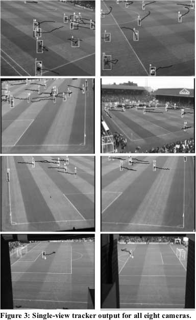
The two-stage method outlined in this paper can be successfully demonstrated in several recorded matches. A live system is being installed and will be available for testing soon. The output from the second stage tracking process is shown in Fig. 5; given the Feature input from the eight cameras shown in Fig. 3.
The system works as planned and gives reasonably reliable and accurate results. Work is currently being undertaken to provide a quantitative evaluation of these results.

Match situations involving many tightly packed players give inaccurate estimates, and re-initialisation errors as the players re-disperse. In the limiting case, these situations are probably insoluble. In general, several system components, discussed below, critically affect the performance of the system.
Firstly, the consistency of the camera homography is very important. If there are systematic errors between specific cameras, the data association step is less likely to be correct. If the error cannot be removed then an empirical correction is acceptable. Secondly, the single view tracker is designed to output one measurement per player observed in that camera. Currently, if two players enter its field of view as an occluded group, there is no mechanism for the single-view tracker to recognise the correct number of players. This could be facilitated by feedback from the multi-view tracker. This could be integrated into our architecture quite easily. Finally, there are several ways to improve the data association step, e.g. allowing for a probabilistic association matrix β i , more informed covariance estimates R, and also incorporating the category estimate of the measurement, c.
To conclude, an architecture has been presented to facilitate the modelling of football players using object detection and tracking with single and then multiple cameras
This work is part of the INMOVE project, supported by the European Commission IST 2001-37422. The project partners are: INMOVE Consortium: Technical Research Centre of Finland, Oy Radiolinja Ab, Mirasys Ltd, Netherlands Organization for Applied Scientific Research TNO, University of Genova, Kingston University, IPM Management A/S and ON-AIR A/S
[1] T. Bebie and H. Bieri, ‘SoccerMan: reconstructing soccer games from video sequences’, Proc. ICIP, pp. 898-02, (1998)
[2] Y. Bar-Shalom and X. R. Li, Multitarget-Multisensor Tracking: Priciples and Techniques, YBS, (1995).
[3] A. Criminisi, I. Reid, and A. Zisserman, “A plane measuring device,” Proc. BMVC, (1997).
[4] S. S. Intille and A. F. Bobick, ‘Closed-world tracking’, Proc. ICCV, pp. 672-678, (1995).
[5] T. Kawashima, K. Yoshino, and Y. Aoki, ‘Qualitative Image Analysis of Group Behaviour’, CVPR, pp. 690-3, (1994).
[6] Y. Seo, S. Choi, H. Kim and K. S. Hong, ‘Where are the ball and players?: Soccer game analysis with color- based tracking and image mosaick’, Proc. ICIAP, pp. 196-203, (1997).
[7] R. Tsai, ‘An efficient and accurate camera calibration technique for 3D Machine Vision’, Proc. CVPR, pp. 323-344, (1986).
[8] M. Xu and T. Ellis, ‘Partial observation vs. blind tracking through occlusion’, Proc. BMVC, pp. 777-786, (2002).