Modeling Dynamic Systems
Авторы: The MathWorks
Источник:
The
MathWorks User's Guide
Block Diagram Semantics
A classic block diagram model of a dynamic system graphically consists of blocks and lines (signals). The history of these block diagram models is derived from engineering areas such as Feedback Control Theory and Signal Processing. A block within a block diagram defines a dynamic system in itself. The relationships between each elementary dynamic system in a block diagram are illustrated by the use of signals connecting the blocks. Collectively the blocks and lines in a block diagram describe an overall dynamic system.
The Simulink product extends these classic block diagram models by introducing the notion of two classes of blocks, nonvirtual blocks and virtual blocks. Nonvirtual blocks represent elementary systems. Virtual blocks exist for graphical and organizational convenience only: they have no effect on the system of equations described by the block diagram model. You can use virtual blocks to improve the readability of your models.
In general, blocks and lines can be used to describe many "models of computations." One example would be a flow chart. A flow chart consists of blocks and lines, but one cannot describe general dynamic systems using flow chart semantics.
The term "time-based block diagram" is used to distinguish block diagrams that describe dynamic systems from that of other forms of block diagrams, and the term block diagram (or model) is used to refer to a time-based block diagram unless the context requires explicit distinction.
To summarize the meaning of time-based block diagrams:
- Simulink block diagrams define time-based relationships between signals and state variables. The solution of a block diagram is obtained by evaluating these relationships over time, where time starts at a user specified "start time" and ends at a user specified "stop time." Each evaluation of these relationships is referred to as a time step.
- Signals represent quantities that change over time and are defined for all points in time between the block diagram's start and stop time.
- The relationships between signals and state variables are defined by a set of equations represented by blocks. Each block consists of a set of equations (block methods). These equations define a relationship between the input signals, output signals and the state variables. Inherent in the definition of a equation is the notion of parameters, which are the coefficients found within the equation.
Creating Models
The Simulink product provides a graphical editor that allows you to create and connect instances of block types selected from libraries of block types via a library browser. Libraries of blocks are provided representing elementary systems that can be used as building blocks. The blocks supplied with Simulink are called built-in blocks. Users can also create their own block types and use the Simulink editor to create instances of them in a diagram. User-defined blocks are called custom blocks.
Time
Time is an inherent component of block diagrams in that the results of a block diagram simulation change with time. Put another way, a block diagram represents the instantaneous behavior of a dynamic system. Determining a system's behavior over time thus entails repeatedly solving the model at intervals, called time steps, from the start of the time span to the end of the time span. The process of solving a model at successive time steps is referred to as simulating the system that the model represents.
States
Typically the current values of some system, and hence model, outputs are functions of the previous values of temporal variables. Such variables are called states. Computing a model's outputs from a block diagram hence entails saving the value of states at the current time step for use in computing the outputs at a subsequent time step. This task is performed during simulation for models that define states.
Two types of states can occur in a Simulink model: discrete and continuous states. A continuous state changes continuously. Examples of continuous states are the position and speed of a car. A discrete state is an approximation of a continuous state where the state is updated (recomputed) using finite (periodic or aperiodic) intervals. An example of a discrete state would be the position of a car shown on a digital odometer where it is updated every second as opposed to continuously. In the limit, as the discrete state time interval approaches zero, a discrete state becomes equivalent to a continuous state.
Blocks implicitly define a model's states. In particular, a block that needs some or all of its previous outputs to compute its current outputs implicitly defines a set of states that need to be saved between time steps. Such a block is said to have states.
The following is a graphical representation of a block that has states:
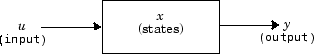
Blocks that define continuous states include the following standard Simulink blocks:
- Integrator
- State-Space
- Transfer Fcn
- Variable Transport Delay
- Zero-Pole
The total number of a model's states is the sum of all the states defined by all its blocks. Determining the number of states in a diagram requires parsing the diagram to determine the types of blocks that it contains and then aggregating the number of states defined by each instance of a block type that defines states. This task is performed during the Compilation phase of a simulation.
Working with States
The following facilities are provided for determining, initializing, and logging a model's states during simulation:
- The model command displays information about the states defined by a model, including the total number of states defined by the model, the block that defines each state, and the initial value of each state.
- The Simulink debugger displays the value of a state at each time step during a simulation, and the Simulink debugger's states command displays information about the model's current states.
- The Data Import/Export pane of a model's Configuration Parameters dialog box allows you to specify initial values for a model's states, and to record the values of the states at each time step during simulation as an array or structure variable in the MATLAB workspace.
- The Block Parameters dialog box (and the ContinuousStateAttributes parameter) allows you to give names to states for those blocks (such as the Integrator) that employ continuous states. This can simplify analyzing data logged for states, especially when a block has multiple states.
Continuous States
Computing a continuous state entails knowing its rate of change, or derivative. Since the rate of change of a continuous state typically itself changes continuously (i.e., is itself a state), computing the value of a continuous state at the current time step entails integration of its derivative from the start of a simulation. Thus modeling a continuous state entails representing the operation of integration and the process of computing the state's derivative at each point in time. Simulink block diagrams use Integrator blocks to indicate integration and a chain of blocks connected to an integrator block's input to represent the method for computing the state's derivative. The chain of blocks connected to the integrator block's input is the graphical counterpart to an ordinary differential equation (ODE).
In general, excluding simple dynamic systems, analytical methods do not exist for integrating the states of real-world dynamic systems represented by ordinary differential equations. Integrating the states requires the use of numerical methods called ODE solvers. These various methods trade computational accuracy for computational workload. The Simulink product comes with computerized implementations of the most common ODE integration methods and allows a user to determine which it uses to integrate states represented by Integrator blocks when simulating a system.
Computing the value of a continuous state at the current time step entails integrating its values from the start of the simulation. The accuracy of numerical integration in turn depends on the size of the intervals between time steps. In general, the smaller the time step, the more accurate the simulation. Some ODE solvers, called variable time step solvers, can automatically vary the size of the time step, based on the rate of change of the state, to achieve a specified level of accuracy over the course of a simulation. The user can specify the size of the time step in the case of fixed-step solvers, or the solver can automatically determine the step size in the case of variable-step solvers. To minimize the computation workload, the variable-step solver chooses the largest step size consistent with achieving an overall level of precision specified by the user for the most rapidly changing model state. This ensures that all model states are computed to the accuracy specified by the user.
Discrete States
Computing a discrete state requires knowing the relationship between its value at the current time step and its value at the previous time step. This is referred to this relationship as the state's update function. A discrete state depends not only on its value at the previous time step but also on the values of a model's inputs. Modeling a discrete state thus entails modeling the state's dependency on the systems' inputs at the previous time step. Simulink block diagrams use specific types of blocks, called discrete blocks, to specify update functions and chains of blocks connected to the inputs of discrete blocks to model the dependency of a system's discrete states on its inputs.
As with continuous states, discrete states set a constraint on the simulation time step size. Specifically, the step size must ensure that all the sample times of the model's states are hit. This task is assigned to a component of the Simulink system called a discrete solver. Two discrete solvers are provided: a fixed-step discrete solver and a variable-step discrete solver. The fixed-step discrete solver determines a fixed step size that hits all the sample times of all the model's discrete states, regardless of whether the states actually change value at the sample time hits. By contrast, the variable-step discrete solver varies the step size to ensure that sample time hits occur only at times when the states change value.
Modeling Hybrid Systems
A hybrid system is a system that has both discrete and continuous states. Strictly speaking, any model that has both continuous and discrete sample times is treated as a hybrid model, presuming that the model has both continuous and discrete states. Solving such a model entails choosing a step size that satisfies both the precision constraint on the continuous state integration and the sample time hit constraint on the discrete states. The Simulink software meets this requirement by passing the next sample time hit, as determined by the discrete solver, as an additional constraint on the continuous solver. The continuous solver must choose a step size that advances the simulation up to but not beyond the time of the next sample time hit. The continuous solver can take a time step short of the next sample time hit to meet its accuracy constraint but it cannot take a step beyond the next sample time hit even if its accuracy constraint allows it to.
You can simulate hybrid systems using any one of the integration methods, but certain methods are more effective than others. For most hybrid systems, the Runge-Kutta variable-step methods, ode23 and ode45, are superior to the other solvers in terms of efficiency. Because of discontinuities associated with the sample and hold of the discrete blocks, MathWorks does not recommend the ode15s and ode113 solvers for hybrid systems.
Block Parameters
Key properties of many standard blocks are parameterized. For example, the Constant value of the Simulink Constant block is a parameter. Each parameterized block has a block dialog that lets you set the values of the parameters. You can use MATLAB expressions to specify parameter values. Simulink evaluates the expressions before running a simulation. You can change the values of parameters during a simulation. This allows you to determine interactively the most suitable value for a parameter.
A parameterized block effectively represents a family of similar blocks. For example, when creating a model, you can set the Constant value parameter of each instance of the Constant block separately so that each instance behaves differently. Because it allows each standard block to represent a family of blocks, block parameterization greatly increases the modeling power of the standard Simulink libraries.
Tunable Parameters
Many block parameters are tunable. A tunable parameter is a parameter whose value can be changed without recompiling the model. For example, the gain parameter of the Gain block is tunable. You can alter the block's gain while a simulation is running. If a parameter is not tunable and the simulation is running, the dialog box control that sets the parameter is disabled.
You can not change the values of source block parameters through either a dialog box or the Model Explorer while a simulation is running. Opening the dialog box of a source block with tunable parameters causes a running simulation to pause. While the simulation is paused, you can edit the parameter values displayed on the dialog box. However, you must close the dialog box to have the changes take effect and allow the simulation to continue. The changes take effect at the start of the next time step.
Block Sample Times
Every Simulink block has a sample time which defines when the block will execute . Most blocks allow you to specify the sample time via a SampleTime parameter. Common choices include discrete, continuous, and inherited sample times.
| Common Sample Time Types | Sample Time | Examples |
|---|---|---|
| Discrete | [TS, T0] | Unit Delay, Digital Filter |
| Continuous | [0, 0] | Integrator, Derivative |
| Inherited | [–1, 0] | Gain, Sum |
For discrete blocks, the sample time is a vector [Ts, To] where Ts is the time interval or period between consecutive sample times and To is an initial offset to the sample time. In contrast, the sample times for nondiscrete blocks are represented by ordered pairs that use zero, a negative integer, or infinity to represent a specific type of sample time. For example, continuous blocks have a nominal sample time of [0, 0] and are used to model systems in which the states change continuously (e.g., a car accelerating). Whereas you indicate the sample time type of an inherited block symbolically as [–1, 0] and Simulink then determines the actual value based upon the context of the inherited block within the model.
Note that not all blocks accept all types of sample times. For example, a discrete block cannot accept a continuous sample time.
For a visual aid, Simulink allows the optional color-coding and annotation of any block diagram to indicate the type and speed of the block sample times. You can capture all of the colors and the annotations within a legend.
Custom Blocks
You can create libraries of custom blocks that you can then use in your models. You can create a custom block either graphically or programmatically. To create a custom block graphically, you draw a block diagram representing the block's behavior, wrap this diagram in an instance of the Simulink Subsystem block, and provide the block with a parameter dialog, using the Simulink block mask facility. To create a block programmatically, you create a MATLAB file or a MEX-file that contains the block's system functions. The resulting file is called an S-function. You then associate the S-function with instances of the Simulink S-Function block in your model. You can add a parameter dialog to your S-Function block by wrapping it in a Subsystem block and adding the parameter dialog to the Subsystem block.
Systems and Subsystems
A Simulink block diagram can consist of layers. Each layer is defined by a subsystem. A subsystem is part of the overall block diagram and ideally has no impact on the meaning of the block diagram. Subsystems are provided primarily to help with the organizational aspects of a block diagram. Subsystems do not define a separate block diagram.
The Simulink software differentiates between two different types of subsystems: virtual and nonvirtual. The primary difference is that nonvirtual subsystems provide the ability to control when the contents of the subsystem are evaluated.
Virtual Subsystems
Virtual subsystems provide graphical hierarchy in models. Virtual subsystems do not impact execution. During model execution, the Simulink engine flattens all virtual subsystems, i.e., Simulink expands the subsystem in place before execution. This expansion is very similar to the way macros work in a programming language such as C or C++. Roughly speaking, there will be one system for the top-level block diagram which is referred to as the root system, and several lower-level systems derived from nonvirtual subsystems and other elements in the block diagram. You will see these systems in the Simulink Debugger. The act of creating these internal systems is often referred to as flattening the model hierarchy.
Nonvirtual Subsystems
Nonvirtual subsystems, which are drawn with a bold border, provide execution and graphical hierarchy in models. Nonvirtual subsystems are executed as a single unit (atomic execution) by the Simulink engine. You can create conditionally executed subsystems that are executed only when a precondition—such as a trigger, an enable, a function-call, or an action— occurs. Simulink always computes all inputs used during the execution of a nonvirtual subsystem before executing the subsystem. Simulink defines the following nonvirtual subsystems.
Atomic subsystems. The primary characteristic of an atomic subsystem is that blocks in an atomic subsystem execute as a single unit. This provides the advantage of grouping functional aspects of models at the execution level. Any Simulink block can be placed in an atomic subsystem, including blocks with different execution rates. You can create an atomic subsystem by selecting the Treat as atomic unit option on a virtual subsystem (see the Atomic Subsystem block for more information).
Enabled subsystems. An enabled subsystem behaves similarly to an atomic subsystem, except that it executes only when the signal driving the subsystem enable port is greater than zero. To create an enabled subsystem, place an Enable Port block within a Subsystem block. You can configure an enabled subsystem to hold or reset the states of blocks within the enabled subsystem prior to a subsystem enabling action. Simply select the States when enabling parameter of the Enable Port block. Similarly, you can configure each output port of an enabled subsystem to hold or reset its output prior to the subsystem disabling action. Select the Output when disabled parameter in the Outport block.
Triggered subsystems. You create a triggered subsystem by placing a trigger port block within a subsystem. The resulting subsystem executes when a rising or falling edge with respect to zero is seen on the signal driving the subsystem trigger port. The direction of the triggering edge is defined by the Trigger type parameter on the trigger port block. Simulink limits the type of blocks placed in a triggered subsystem to blocks that do not have explicit sample times (i.e., blocks within the subsystem must have a sample time of -1) because the contents of a triggered subsystem execute in an aperiodic fashion. A Stateflow chart can also have a trigger port which is defined by using the Stateflow editor. Simulink does not distinguish between a triggered subsystem and a triggered chart.
Function-call subsystems. A function-call subsystem is a subsystem that another block can invoke directly during a simulation. It is analogous to a function in a procedural programming language. Invoking a function-call subsystem is equivalent to invoking the output and update methods of the blocks that the subsystem contains in sorted order. The block that invokes a function-call subsystem is called the function-call initiator. Stateflow, Function-Call Generator, and S-function blocks can all serve as function-call initiators. To create a function-call subsystem, drag a Function-Call Subsystem block from the Ports & Subsystems library into your model and connect a function-call initiator to the function-call port displayed on top of the subsystem. You can also create a function-call subsystem from scratch by first creating a Subsystem block in your model and then creating a Trigger block in the subsystem and setting the Trigger block Trigger type to function-call.
You can configure a function-call subsystem to be triggered (the default) or periodic by setting its Sample time type to be triggered or periodic, respectively. A function-call initiator can invoke a triggered function-call subsystem zero, once, or multiple times per time step. The sample times of all the blocks in a triggered function-call subsystem must be set to inherited (-1).
A function-call initiator can invoke a periodic function-call subsystem only once per time step and must invoke the subsystem periodically. If the initiator invokes a periodic function-call subsystem aperiodically, Simulink halts the simulation and displays an error message. The blocks in a periodic function-call subsystem can specify a noninherited sample time or inherited (-1) sample time. All blocks that specify a noninherited sample time must specify the same sample time, that is, if one block specifies .1 as its sample time, all other blocks must specify a sample time of .1 or -1. If a function-call initiator invokes a periodic function-call subsystem at a rate that differs from the sample time specified by the blocks in the subsystem, Simulink halts the simulation and displays an error message.
Enabled and triggered subsystems. You can create an enabled and triggered subsystem by placing a Trigger Port block and an Enable Port block within a Subsystem block. The resulting subsystem is essentially a triggered subsystem that executes when the subsystem is enabled and a rising or falling edge with respect to zero is seen on the signal driving the subsystem trigger port. The direction of the triggering edge is defined by the Trigger type parameter on the trigger port block. Because the contents of a triggered subsystem execute in an aperiodic fashion, Simulink limits the types of blocks placed in an enabled and triggered subsystem to blocks that do not have explicit sample times. In other words, blocks within the subsystem must have a sample time of -1).
Action subsystems. Action subsystems can be thought of as an intersection of the properties of enabled subsystems and function-call subsystems. Action subsystems are restricted to a single sample time (e.g., a continuous, discrete, or inherited sample time). Action subsystems must be executed by an action subsystem initiator. This is either an If block or a Switch Case block. All action subsystems connected to a given action subsystem initiator must have the same sample time. An action subsystem is created by placing an Action Port block within a Subsystem block. The subsystem icon will automatically adapt to the type of block (i.e., If or Switch Case block) that is executing the action subsystem.
Action subsystems can be executed at most once by the action subsystem initiator. Action subsystems give you control over when the states reset via the States when execution is resumed parameter on the Action Port block. Action subsystems also give you control over whether or not to hold the outport values via the Output when disabled parameter on the outport block. This is analogous to enabled subsystems.
Action subsystems behave very similarly to function-call subsystems because they must be executed by an initiator block. Function-call subsystems can be executed more than once at any given time step whereas action subsystems can be executed at most once. This restriction means that a larger set of blocks (e.g., periodic blocks) can be placed in action subsystems as compared to function-call subsystems. This restriction also means that you can control how the states and outputs behave.
While iterator subsystems. A while iterator subsystem will run multiple iterations on each model time step. The number of iterations is controlled by the While Iterator block condition. A while iterator subsystem is created by placing a While Iterator block within a subsystem block.
A while iterator subsystem is very similar to a function-call subsystem in that it can run for any number of iterations at a given time step. The while iterator subsystem differs from a function-call subsystem in that there is no separate initiator (e.g., a Stateflow Chart). In addition, a while iterator subsystem has access to the current iteration number optionally produced by the While Iterator block. A while iterator subsystem also gives you control over whether or not to reset states when starting via the States when starting parameter on the While Iterator block.
For iterator subsystems. A for iterator subsystem will run a fixed number of iterations at each model time step. The number of iterations can be an external input to the for iterator subsystem or specified internally on the For Iterator block. A for iterator subsystem is created by placing a For Iterator block within a subsystem block.
A for iterator subsystem has access to the current iteration number that is optionally produced by the For Iterator block. A for iterator subsystem also gives you control over whether or not to reset states when starting via the States when starting parameter on the For Iterator block. A for iterator subsystem is very similar to a while iterator subsystem with the restriction that the number of iterations during any given time step is fixed.
For each subsystems. The for each subsystem allows you to repeat an algorithm for individual elements (or subarrays) of an input signal. Here, the algorithm is represented by the set of blocks in the subsystem and is applied to a single element (or subarray) of the signal. You can configure the decomposition of the subsystem inputs into elements (or subarrays) using the For Each block, which resides in the subsystem. The For Each block also allows you to configure the concatenation of individual results into output signals. An advantage of this subsystem is that it maintains separate sets of states for each element or subarray that it processes. In addition, for certain models, the for each subsystem improves the code reuse of the code generated by Simulink Coder.
Signals
The term signal refers to a time varying quantity that has values at all points in time. You can specify a wide range of signal attributes, including signal name, data type (e.g., 8-bit, 16-bit, or 32-bit integer), numeric type (real or complex), and dimensionality (one-dimensional, two-dimensional, or multidimensional array). Many blocks can accept or output signals of any data or numeric type and dimensionality. Others impose restrictions on the attributes of the signals they can handle.
On the block diagram, signals are represented with lines that have an arrowhead. The source of the signal corresponds to the block that writes to the signal during evaluation of its block methods (equations). The destinations of the signal are blocks that read the signal during the evaluation of the block's methods (equations).
A good way to understand the definition of a signal is to consider a classroom. The teacher is the one responsible for writing on the white board and the students read what is written on the white board when they choose to. This is also true of Simulink signals: a reader of the signal (a block method) can choose to read the signal as frequently or infrequently as so desired.
Block Methods
Blocks represent multiple equations. These equations are represented as block methods. These block methods are evaluated (executed) during the execution of a block diagram. The evaluation of these block methods is performed within a simulation loop, where each cycle through the simulation loop represents the evaluation of the block diagram at a given point in time.
Method Types
Names are assigned to the types of functions performed by block methods. Common method types include:
- Outputs
Computes the outputs of a block given its inputs at the current time step and its states at the previous time step. - Update
Computes the value of the block's discrete states at the current time step, given its inputs at the current time step and its discrete states at the previous time step. - Derivatives
Computes the derivatives of the block's continuous states at the current time step, given the block's inputs and the values of the states at the previous time step.
Method Naming Convention
Block methods perform the same types of operations in different ways for different types of blocks. The Simulink user interface and documentation uses dot notation to indicate the specific function performed by a block method:
BlockType.MethodType
For example, the method that computes the outputs of a Gain block is referred to as
Gain.Outputs
The Simulink debugger takes the naming convention one step further and uses the instance name of a block to specify both the method type and the block instance on which the method is being invoked during simulation, e.g.,
g1.Outputs
Model Methods
In addition to block methods, a set of methods is provided that compute the model's properties and its outputs. The Simulink software similarly invokes these methods during simulation to determine a model's properties and its outputs. The model methods generally perform their tasks by invoking block methods of the same type. For example, the model Outputs method invokes the Outputs methods of the blocks that it contains in the order specified by the model to compute its outputs. The model Derivatives method similarly invokes the Derivatives methods of the blocks that it contains to determine the derivatives of its states.