Determining Optical Flow
Автор: Berthold K.P. Horn, Brian G. Rhunck
Источник: Artificial Intelligence Laboratory, Massachusetts Institute of Technology, Cambridge, MA 02139, U.S.A.
Introduction
Optical flow is the distribution of apparent velocities of movement of brightness patterns in an image. Optical flow can arise from relative motion of objects and the viewer. Consequently, optical flow can give important information about the spatial arrangement of the objects viewed and the rate of change of this arrangement. Discontinuities in the optical flow can help into segmenting images into regions that correspond to different objects. I Attempts have been made to perform such segmentation using differences between successive image frames. Several papers address the problem of recovering the motions of objects relative to the viewer from the optical flow. Some recent papers provide a clear exposition of this enterprise. The mathematics can be made rather difficult, by the way, by choosing an inconvenient coordinate system. In some cases information about the shape of an object may also be recovered. These papers begin by assuming that the optical flow has already been determined. Although some reference has been made to schemes for computing the flow from successive views of a scene, the specifics of a scheme for determining the flow from the image have not been described. Related work has been done in an attempt to formulate a model for the short range motion detection processes in human vision. The pixel recursive equations of Netravali and Robbins, designed for coding motion in television signals, bear some similarity to the iterative equations developed in this paper. A recent review of computational techniques for the analysis of image sequences contains over 150 references.
The optical flow cannot be computed at a point in the image independently of neighboring points without introducing additional constraints, because the velocity field at each image point has two components while the change in image brightness at a point in the image plane due to motion yields only one constraint. Consider, for example, a patch of a pattern where brightness varies as a function of one image coordinate but not the other. Movement of the pattern in one direction alters' the brightness at a particular point, but motion in the other direction yields no change. Thus components of movement in the latter direction cannot be determined locally.
Relationship to Object Motion
The relationship between the optical flow in the image plane and the velocities of objects in the three dimensional world is not necessarily obvious. We perceive motion when a changing picture is projected onto a stationary screen,for example. Conversely, a moving object may give rise to a constant brightness pattern. Consider, for example, a uniform sphere which exhibits shading because its surface elements are oriented in many different directions. Yet, when it is rotated, the optical flow is zero at all points in the image, since the shading does not move with the surface. Also, specular reflections move with a velocity characteristic of the virtual image, not the surface in which light is reflected.
For convenience, we tackle a particularly simple world where the apparent velocity of brightness patterns can be directly identified with the movement of surfaces in the scene.
The Restricted Problem Domain
To avoid variations in brightness due to shading effects we initially assume that the surface being imaged is flat. We further assume that the incident illumination is uniform across the surface. The brightness at a point in the image is then proportional to the reflectance of the surface at the corresponding point on the object. Also, we assume at first that reflectance varies smoothly and has nospatial discontinuities. This latter condition assures us that the image brightness is differentiable. We exclude situations where objects occlude one another, in part, because discontinuities in reflectance are found at object boundaries. In two of the experiments discussed later, some of the problems occasioned by occluding edges are exposed.
In the simple situation described, the motion of the brightness patterns in the image is determined directly by the motions of corresponding points on the surface of the object. Computing the velocities of points on the object is a matter of simple geometry once the optical flow is known.
Constraints
We will derive an equation that relates the change in image brightness at a point to the motion of the brightness pattern. Let the image brightness at the point (x, y) in the image plane at time r be denoted by E(x, y, t). Now consider what happens when the pattern moves. The brightness of a particular point in the pattern is constant, so that

Using the chain rule for differentiation we see that,

(See Appendix A for a more detailed derivation.) If we let

then it is easy to see that we have a single linear equation in the two unknowns u and v,

where we have also introduced the additional abbreviations Ex, Ey, and Et, for the partial derivatives of image brightness with respect to x, y and t, respectively. The constraint on the local flow velocity expressed by this equation is illustrated in Fig. 1. Writing the equation in still another way,

Thus the component of the movement in the direction of the brightness gradient (Ex, Ey) equals

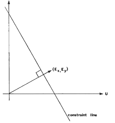
Figure 1 – The basic rate of change of image brightness equation constrains the optical flow velocity.The velocity (u, v ) has to lie along a line perpendicular to the brightness gradient vector (Ex, Ey).The distance of this line from the origin equals Et divided by the magnitude of (Ex, Ey).
We cannot, however, determine the component of the movement in the direction of the iso-brightness contours, at right angles to the brightness gradient. As a consequence, the flow velocity (u, v) cannot be computed locally without introducing additional constraints.
Summary
A method has been developed for computing optical flow from a sequence of images. It is based on the observation that the flow velocity has two components and that the basic equation for the rate of change of image brightness provides only one constraint. Smoothness of the flow was introduced as a second constraint. An iterative method for solving the resulting equation was then developed. A simple implementation provided visual confirmation of convergence of the solution in the form of needle diagrams. Examples of several different types of optical flow patterns were studied. These included cases where the Laplacian of the flow was zero as well as cases where it became infinite at singular points or along bounding curves.
The computed optical flow is somewhat inaccurate since it is based on noisy, quantized measurements. Proposed methods for obtaining information about the shapes of objects using derivatives (divergence and curl) of the optical flow field may turn out to be impractical since the inaccuracies will be amplified.
References
1. I . Ames. W.F., Numerical Methods for Partial Differential Equations (Academic Press, New York.1977).2. Batali. I. and Ullman. S., Motion detection and analysis. Roc. of the ARPA Image Understanding Workshop. 7-8 November 1979 (Science Applications Inc.. Arlington. VA 1979) pp. 69-75.
3. Clocksin. W.. Determining the orientation of surfaces from optical flow. Roc. of the Third AISB Conference. Hamburg (1978) pp. 93-102.
4. Conte. S.D. and de Boor. C.. Elementary Numerical Analysis (McGraw-Hill. New York, 1965, 1972).
5.Fennema. C.L. and Thompson. W.B.. Velocity determination in scenes containing several moving objects. Computer Graphics and Image Processing 9 (4) (1979) 301-315.