
Abstract on a subject of a master's thesis
"Optimization of the Optimistic Protocol – Overview"
Content
- Introduction
- 1 Reducing the cost of rollback
- 2 Reduction the memory usage
- 2.1 State saving optimization
- 3 Optimism control
- 3.1 Non-adaptive protocols
- 3.2 Adaptive protocols based on local states
- 3.3 Adaptive protocols based on global state
- 3.4 Adaptive protocols based on probabilistic calculations
- 3.5 Other adaptive protocols
- 4 Evolutionary approaches
- 5 Algorithms for the global virtual time computing
- 5.1 Centralized GVT computing
- 5.2 Distributed GVT computing
- 6 Classification of algorithms for optimistic protocol optimization
- References
Introduction
Parallel discrete-event simulation (PDES) is performed by a set of logical processes (LP) that communicate to each other by passing timestamped messages representing the simulation events. Each LP has its own local clock, also called local virtual time (LVT), to indicate the progress of simulation. The LVT is advanced whenever an event is executed in the LP, and the parallel simulation is complete when all LVTs reach the duration of simulation. Two PDES mechanisms have been widely discussed: conservative and optimistic. The conservative approach ensures that an event execution will not cause any causality error before it is carried out. On the other hand, the optimistic approach performs the event execution greedily without adhering to the safety constraint.
Optimistic methods allow violations to occur, but are able to detect and recover from them. Optimistic approaches offer two important advantages over conservative techniques. First, they can exploit greater degrees of parallelism. Second, conservative mechanism generally rely on application specific information (e.g., distance between objects) in order to determine which events are safe to process. While optimistic mechanisms can execute more efficiently if they exploit such information, they are less reliant on such information for correct execution. On the other hand, optimistic methods may require more overhead computations than conservative approaches, leading to certain performance degradations.
The Time Warp mechanism is the most well-known optimistic algorithm. The principle of his work lies in the implementation of events without assurance of compliance with the natural order. If there is a violation of the natural order of time stamps of events, the protocol rolls back to the desired state through the mechanism of anti-messages. Anti-message – is a duplicate of the previously sent message. The main disadvantages of the Time Warp algorithm is excessive memory consumption, the possibility of cascading rollbacks, low speed simulation in case of frequent rollbacks. The following describes the existing algorithms for optimizing Time Warp, which trying to address these shortcomings.
1 Reducing the cost of rollback
Aggressive cancellation on rollback makes the assumption that most of the output values will change when executing back to the local virtual time before rollback was caused. To do this, all anti-messages are generated when rolling back, before any re-execution of events is done [2]. Lazy cancellation on rollback, makes the assumption that little if any of the output will change if a new event is added to the sequence. This technique is effective, but it has the potential to cause larger rollbacks on dependant processes by letting them execute further in virtual time before being corrected [1,2]. Lazy re-evaluation is somewhat similar to lazy cancellation, but deals with the delayed discarding of state vectors instead of the delayed sending of antimessages. Adaptive cancellation designed to solve the problem the need to define a cancellation strategy at the startup phase. It allows a process to decide which strategy to use the cancellation, based on run-time performance [1,2]. Fujimoto proposed a direct cancellation mechanism that uses shared memory to optimize the cancellation of incorrect computations. If during the execution of an event E1 a new event E2 is scheduled, the mechanism associates a pointer reference to E2 with event E1. Upon rollback of event E1, the pointer reference can be used to cancel E2, using either lazy or aggressive cancellation [2,3].
Other approaches have been proposed for the earlier limit the rollback chains. Prakash and Subramanian [2] attach some state information to messages, to prevent cascading rollbacks. Madisetti [2] proposed within their Wolf system a mechanism that freezes the spatial spreading of the incorrect computation based upon a so-called sphere of influence. A disadvantage of this approach is that the set of simulation processes that might be affected by the incorrect computation is significantly larger than the actual set, and thereby leads to sending unnecessary control messages [2].
2 Reduction the memory usage
The mechanism of Pruneback [5] Preiss & Loucks proposed to use to handle memory usage when the system was at or near the limit for available memory. The Pruneback mechanism is based upon recovering needed memory from the saved state information of the physical process. If a rollback occurs to the now missing state, it ends up rolling back to a the first virtual time state before the missing state, and then coasting forward using the saved input events to recalculate that state. There are constraints to pruning back. Neither the physical processes nor the GVT state are to be pruned [4]. Carothers [4,6] applied the approach for correction the physical processes as potentially reversible. Rollback is achieved by using reverse computations using the current state and the stored input events.
2.1 State saving optimization
The periodic state saving (PSS) method reduces the state saving overhead by increasing the checkpoint interval. PSS copies the entire state only after every χ-th state update, where χ is the state saving interval. If a rollback occurs and the required state is not in the state queue, the LP must roll back to an earlier checkpointed state [7]. The checkpoint interval is the key parameter that determines the efficiency of PSS method: it regulates the trade-off between the total cost of state saving and the amount of re-execution in coasting forward. Fleischmann and Wilsey [7] performed an empirical study on four adaptive PSS methods. They present a heuristic that recalculates the state saving costs (state saving and coasting forward) after every N events. If the execution time has increased significantly, the state saving interval is decreased by one, otherwise it is increased by one. Sköld and Rönngren argued that the optimal checkpoint interval also depends on the execution time or event granularity for different types of events. Their event sensitive state saving method is sensitive to which type of event the previously executed event belongs, and decide whether to save the state vector based on this information.
Francesco Quaglia proposed the algorithm for sparse state saving based on the history of events [8]. The essence of the algorithm is that each LP is trying to predict intervals of virtual time, that there will rollback. This approach is also based on monitoring the cost function of checkpoint and rollback, which is used to recalculate the dynamic allocation parameter that determines the percentage of saved states. Incremental State Saving machanism (ISS) usually usues обычно использует partial state update. Incremental saving the history of the LP states is created by saving the old value of the variable before it is overwritten and the new value that is used to rollback – restore the value of each stored in reverse order of preservation. To improve methods of PSS and ISS were proposed hybrid methods that alternate between these two mechanisms. Francesco Quaglia [9] proposed hybrid approach based on the combination of the PSS and ISS. This approach offers a process to periodically save the state, and to keep part of the inverse transformations between checkpoints. Adjustable parameters are the size of the interval and the number of partial saved states for the interval between two checkpoints.
3 Optimism control
3.1 Non-adaptive protocols
The first method for the excessive optimism control uses time windows. This approach limits the optimism, performing only in the event modeling within the time window. The first protocol that uses this technique is Moving Time Window (MTW). The key problem – the most appropriate time window size. A similar idea was explored Turner and Xu [10] in the protocol Bounded Time Warp (BTW), where no events are processed until all the processes have not reached the time of new bound is established.
The Breathing Time Bucket algorithm uses optimistic processing with local rollback. However, unlike other optimistic windowing approaches, anti-messages are never required. In other words, Breathing Time Buckets could be classified as a risk-free optimistic approach. Breathing Time Warp [11] is an extension to the Breathing Time Bucket algorithm by allowing it to take risks. The idea is to execute the first N1 events beyond the GVT, just as the basic Time Warp algorithm does. Then the protocol issues a nonblocking synchronization operation and switches back to the risk-free breathing time bucket algorithm to execute the next N2 events. If all LPs reached their event horizon, that is, issued the nonblocking synchronization, a new GVT computation is started and a next cycle is issued.
3.2 Adaptive protocols based on local states
The control mechanism in Adaptive Time Warp [12] uses a penalty based method to limit optimism by blocking the LP for an interval of real time (the blocking window). The blocking window is adjusted to minimize the sum of total CPU time spent in blocked state and recovery state. The logical process may decide to temporarily suspend event processing if it had recently experienced an abnormally high number of causality errors.
Hamnes and Tripathi [13] proposed a local adaptive protocol that uses simple local statistical data to avoid additional communication overhead. The protocol is designed to adapt to the application in order to maximize progress of simulation time in real time (with simulation time progress rate α). The algorithm gathers statistics on a per channel basis within each LP and uses this information to maximize α. The probabilistic adaptive direct optimism control [14] is similar in spirit, but adds a probabilistic component in the sense that blocking is induced with a certain probability.
Parameterized Time Warp [15] combines three adaptive mechanisms (state saving period, bounded time window, and scheduling priority) to minimize overhead and increase the performance of the parallel simulation. The measure useful work is defined to determine the actual amount of optimism utilized by the process. Useful work is a function of a number of parameters such as the ratio of the number of committed to the total number of events executed, the number of rollbacks, the number of anti-messages, the rollback length, etc. The state saving period and the bounded time window are increased for larger values of the useful work parameter.
3.3 Adaptive protocols based on global state
The Adaptive Memory Management protocol uses an indirect approach to control overly optimistic event execution. The adaption algorithm attempts to minimize the total execution time rather than concentrating on one specific criteria. It is argued that this approach prevents from optimizing for one aspect of the computation at the expense of a disproportional increase in another.
The Near Perfect State Information (NPSI) protocols [16] are a class of adaptive protocols relying on the availability of near-perfect information on the global state of the parallel simulation. NPSI protocols use a quantity error potential (EPi) associated with each LPi, to control LPi’s optimism. The protocol keeps each EPi up to date as the simulation progresses. A second component of the protocol translates the EPi into control over the aggressiveness and risk of LPi. One instance of a NPSI protocol is the Elastic Time Algorithm (ETA). In ETA, the farther LPi moves away from its predecessor, the slower its progress due to the restraining pull of the elastic band tying it to its predecessor—hence elastic time. The tension in the elastic band corresponds to the LPi’s error potential.
The protocol based on the mechanism of a moving window in computer networks, where the sender and the recipient govern with the help of specific messages a window size has been proposed by Kiran и Fujimoto [17]. They estimate the number of unprocessed messages scheduled for each processor, these estimates are used to determine a moving window, which defines the upper limit of the number of unprocessed messages that the LP can schedule at one time. Progress of GVT commits messages allowing to send more messages. Three steps to estimate the size of the window are applied. The first – an instant window size required for the corresponding serial execution. The second – a window that is required to calculate the following GVT. The third part – the window for optimistic calculations.
3.4 Adaptive protocols based on probabilistic calculations
The MIMDIX system employs the ideas of probabilistic resynchronization to eliminate overly optimistic behavior. A special process called a "genie" probabilistically sends a synchronization message to all LPs, causing them to synchronize to the timestamp of the message. By keeping the timestamp of the synchronization message close to the GVT, the LPs can be kept temporally close to each other, thus reducing the risk of cascading rollbacks.
Damani, Wang and Garg [18] offered parametric algorithm for state reconstruction, where K is a parameter that determines degree of optimism that is used to adjust the optimal balance between efficiency and recovery overhead. K is integer in the range from 0 to N, where N is the total number of processes. It is defined as the maximum number of processes whose failure can cancel some message m.
3.5 Other adaptive protocols
Damani and colleagues [19] offered an optimistic algorithm for a quick stop of erroneous calculations. This algorithm is a modification of Distributed recovery with K-optimistic logging [18]. The scheme does not require a queue of outgoing messages, and anti-messages. It reduces memory overhead and leads to a simple memory management algorithms. The scheme also eliminates the problem of cascading rollbacks that leads to faster simulation. It is used an aggressive cancellation.
The concept of the algorithm is creation and maintenance of information transitive dependencies between processes. Supported by a table of incarnation numbers – the number of rollbacks produced by the process. The table also stores the timestamp message that caused the rollback. If the process discovers that he has received a strangler, it sends a message containing the current incarnation number k and timestamp of the t-th message, and then blocks its work. Broadcasted messages show that all states of k-th incarnation with the virtual time larger then t, are incorrect. The states that depend on them are incorrect too.
Smith, Johnson, and Tygar [20] suggested the completely asynchronous optimistic recovery protocol with minimal rollbacks, based on the method of Optimistic Message Logging. The protocol does not require sending any messages, and reduces the maximum number of rollbacks for each process to one. There are two types of messages, each with its own preservation interval – user (modeling messages) and system messages. Only user messages are logged. Also, the state vector is used for fast loading the desired state.
4 Evolutionary approaches
Evolutionary approaches are relatively new optimization techniques of Time Warp algorithm. The algorithms based on the theory of evolution find the optimal solution by trial and error. Evolutionary algorithms start with a choice of arbitrary solution from the solution space. The suitability of each candidate from a population estimated to select candidates for breeding. Then a pair of candidates are selected and recombination operation is carried out – the creation of offspring. After the children's estimation selection process is repeated to creates the following generation.
The GVA algorithm (Genetic Modifying Algorithm) [21] solves the problem of setting the adaptive parameters that define the mode of recording and recovery. These parameters correspond to the current logging mode (incremental or non-incremental) and the current logging interval. Logging modes and intervals associated with a set of modeling object – genotype. Posterity is estimated using survival function based on the number of committed events. When there is increased productivity, mutations are applied to those parts of the genotype, which were not affected by step of evolution. When the deterioration is detected, a snapshot of the genotype restores to the latter mutations, and mutations in it are renewed. Genotype starts with a random configuration.
Another genetic algorithm is proposed by Wang and Tropper [22] to limit optimism. The algorithm defines an iterative method of optimal window size for event execution. Each processor has its own window size. Estimation of windows is based on the progress of modeling. The windows are estimated at intervals of ten consecutive GVT and survival rate is the mean of ten estimates. Parents are selected either by generating random numbers in the range [0,1] or by stochastic universal sampling, where a random number is generated in the range [0, 1/s], where c is the total number of candidates.
5 Algorithms for the global virtual time computing
The Global Virtual Time (GVT) is used in the parallel optimistic Time Warp synchronization mechanism to determine the progress of the simulation. Contrary to LVT, the essential property of the GVT is that its value is nondecreasing over real time (wall-clock time). Two important problems solved by GVT are fossil collection and committing of irrevocable operations.
5.1 Centralized GVT computing
In centralized GVT algorithms the GVT is computed by a central GVT manager that broadcasts a request to all LPs for their current LVT and while collecting those values perform a min-reduction (global reduce operation selecting the minimum value). In this approach there are two main problems that complicate the computation of an accurate GVT estimation. First, the messages in transit that can potentially roll back a reported LVT, are not taken into consideration; this is also known as the transient message problem. Second, the reported LVT values were drawn from the LPs at different real times, this is called the simultaneous reporting problem.
One of the first GVT algorithms proposed by Samadi [23] starts a GVT computation via a central GVT manager which sends out a GVT start message. After all LPs have send a reply to the request, the GVT manager computes and broadcasts the new GVT value. The transient message problem is solved by acknowledging every message, and reporting the minimum over all timestamps of unacknowledged messages and the LVT of the LP to the GVT manager. Lin and Lazowska [24] introduced some improvements over Samadi’s algorithm. In Lin’s algorithm, the messages are not acknowledged but the message headers include a sequence number. The receiving LP can identify missing messages as gaps in the arriving sequence numbers. The simultaneous reporting problem is solved in the GVT algorithms described above by setting a lower and upper bound on the reporting real time at each LP. Each LP can then forward information to the GVT manager as it leaves the interval.
To reduce the communication complexity of the GVT computation, Bellenot [25] uses a message routing graph. The GVT computation requires two cycles, one to start the GVT computation and the second to report local minima and compute the global minimum. The multi-level token passing algorithm proposed by Concepcion and Kelly [26] applies a hierarchical method to parallelize the GVT computation. The multi-level decomposition allows the parallel determination of the minimum time among the managers of each level.
Bauer et al. [27] proposed an efficient algorithm where all event messages through a certain communication channel are numbered. The LPs administer the number of messages sent and received, and the minimum timestamp of an event message since the last GVT report. Periodically, the LPs send their local information and their LVT to the GVT manager, which deduces from the information the minimum of the transient message timestamps and LVTs.
The passive response GVT (pGVT) algorithm [28] is able to operate in an environment with faulty communication channels, and adapts to the performance capabilities of the parallel system on which it executes. In the pGVT algorithm, the LP considers message latency times to decide when new GVT information should be sent to the GVT manager. This allows each LP to report GVT information to arrive just in time to allow for aggressive GVT advancement by the GVT manager. A key performance improvement of pGVT is that the LPs simulating along the critical path will more frequently report GVT information than others.
An efficient, asynchronous, shared-memory GVT algorithm is presented by Fujimoto and Hybinette [29]. The GVT algorithm exploits the guarantee of shared-memory multiprocessors that no two processors will observe a set of memory operations as occurring in different orders. algorithm does not require message acknowledgements, FIFO delivery of messages, or special GVT messages.
5.2 Distributed GVT computing
Distributed GVT algorithms neither require a centralized GVT manager, nor the availability of shared-memory between the LPs. Mattern [30] presented an efficient "parallel" distributed snapshot algorithm for non-FIFO communication channels which neither requires messages to be acknowledged. The algorithm determines two snapshots, where the second is pushed forward such that all transient messages are enclosed between the two snapshots. The problem of knowing when the snapshot is complete (all transient messages have been caught) is solved by a distributed termination detection scheme.
Srinivasan and Reynolds [31] designed a parallel reduction network (PRN)—in hardware—used by their GVT algorithm. The LPs communicate some state information to the PRN, which is maintained by the distributed GVT algorithm. Along state information, message receipt acknowledgements are also sent over the PRN. The PRN is used to compute and disseminate the minimum LVT of all LPs and the minimum of the timestamp of all unreceived messages. The GVT is made available to each LP asynchronously of the LPs, at no cost.
The GVT algorithm in the SPEEDES simulation environment is especially optimized to support interactive parallel and distributed optimistic simulation. The transient message problem is solved by flushing out all messages during the GVT update phase. The SPEEDES GVT algorithm continues to process events during this phase, but new messages that might be generated are not immediately released.
6 Classification of algorithms for optimistic protocol optimization
The methods of optimization can be divided into several groups according to solution of problems of the optimistic protocol and ways to achieve results (Fig. 1).
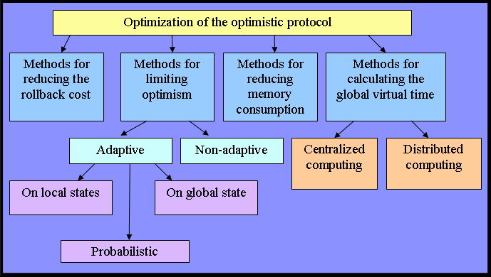
Figure 1 – Classification of methods of optimization optimistic protocol
However, it can not be clearly divided into classes of algorithms, since many of them although they are aimed at improving an efficiency at the same time also affect other aspects of modeling. Fig. 2 shows the causal relationships between the methods and optimization algorithms, as well as between the characteristics of the simulation system.
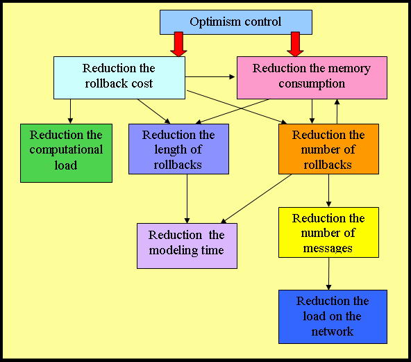
Figure 2 – The causal connection between the classification algorithms
Conclusion
The result of research is the classification algorithms optimized for the type of features and methods used for this purpose, and analysis of algorithms in terms of their strengths and weaknesses and their impact on the optimization of other parameters of the simulation system.
This master's work is not completed yet. Final completion: December 2012. The full text of the work and materials on the topic can be obtained from the author or his head after this date.
References
- Radharamanan Radhakrishnan, Timothy J. McBrayer, Krishnan Subramani, Malolan Chetlur, Vijay Balakrishnan and Philip A. Wilsey. A Comparative Analysis of Various TimeWarp Algorithms Implemented in the WARPED Simulation Kernel. – 1998.
- Voon-Yee Vee, Wen-Jing Hsu. Parallel Discrete Event Simulation: A Survey.
- Richard M. Fujimoto. Parallel discrete event simulation – 1990.
- Bruce Jones, Vanessa Wallace. Time-Event based processing, a Survey.
- Bruno R. Preiss, Wayne M. Loucks. Memory Management Techniques for Time Warp on a Distributed Memory Machine. – 1995.
- Carothers, C., Perumalla, K., Fujimoto, R.M. Efficient Optimistic Parallel Simulations using Reverse Computation. – 2000.
- Josef Fleischmann, Philip A. Wilsey. Comparative Analysis of Periodic State Saving Techniques in Time Warp Simulators. – 1995.
- Francesco Quaglia. Event History Based Sparse State Saving in Time Warp. – 1998.
- Francesco Quaglia. Rollback-based parallel discrete event simulation by using hybrid state saving. – 1997.
- Turner, S.J. and Xu, M.Q. Performance evaluation of the bounded Time Warp algorithm. – 1992.
- Jeff S. Steinman. Breathing Time Warp. – 1992.
- Ball, D. and Hoyt, S. The adaptive Time-Warp concurrency control algorithm. – 1990.
- Hamnes, D. O. and Tripathi, A. Investigations in adaptive distributed simulation. – 1994.
- Alois Ferscha. Probabilistic Adaptive Direct Optimism Control in Time Warp.
- Avinash C. Palaniswamy, Philip A. Wilsey: Parameterized Time Warp (PTW): An Integrated Adaptive Solution to Optimistic PDES. – 1996.
- Srinivasan S., Reynolds P. Elastic Time. – 1998.
- Kiran S. Panesar, Richard M. Fujimoto. Adaptive Flow Control in Time Warp. – 1997.
- Om P. Damani, Yi-Min Wang, Vijay K. Garg. Distributed Recovery with K-Optimistic Logging.
- Om P. Damani, Yi-Min Wang, Vijay K. Garg. Optimistic Distributed Simulation Based on Transitive Dependency Tracking.
- Sean W. Smith, David B. Johnson, and J. D. Tygar. Completely Asynchronous Optimistic Recovery with Minimal Rollbacks. – 1995.
- Alessandro Pellegrini, Roberto Vitali, Francesco Quaglia. An Evolutionary Algorithm to Optimize Log/Restore Operations within Optimistic Simulation Platforms. – 2011.
- Jun Wang, Carl Tropper. Using Genetic Algorithm to Limit the Optimism in Time Warp. – 2009.
- Samadi B. Distributed simulation, algorithms and performance analysis. – 1985, 226 c.
- Yi-Bing Lin, Edward D. Lazowska. Determining the Global Virtual Time in a Distributed Simulation. – 1990.
- Bellenot, S. Global Virtual Time Algorithms. – 1990.
- Conception, A.I., Kelly, S.G., Computing global virtual time using the Multiple-Level Token Passing algorithm. – 1991.
- Bauer, H., Sporrer, C., Distributed logic simulation and an approach to asynchronous GVT-calculation. – 1992.
- D'Souza,L.M., Fan, L.M., Wilsey, P.A. pGvt: An Algorithm for Accurate GVT Estimation. – 1994.
- Richard Fujimoto, Maria Hybinette: Computing Global Virtual Time in Shared-Memory Multiprocessors. – 1997.
- Mattern, F. Efficient algorithms for distributed snapshots and global virtual time approximation. – 1993.
- Srinivasan, S., Reynolgs, P.F. Hardware support for aggressive parallel discrete event simulations. – 1992.