Lossless Wavelet Compression
Авторы: Ian Kaplan
Описание: Рассмотрена концепция целочисленного вейвлет-преобразования без потерь и результаты ее применения на тестовых наборах.
Источник: http://www.bearcave.com/misl/misl_tech/wavelets/compression/
Introduction
This web page discusses lossless data compression using integer to integer wavelet transforms and an integer version of the wavelet packet transform.
The lossless compression discussed here involves 1-D data. However, these algorithms directly generalize to 2-D data (e.g., images) [1]. Applications for lossless compression include compression of experimental data and compression of financial time series (for example, the bid/ask time series that arise from intra-day trading).
Usually a technique like integer to integer wavelet compression is applied to a large data set (like an image) as the first step in the compression process. A second data coding step is applied. Ideally the first step will result in repeated value (either sequential repeats or multiple occurrences of a given value), so additional compression can be achieved by a coding algorithm like Huffman or run length coding.
The motivation behind this web page is not data compression per se. Wavelet compression is a form of predictive compression. Predictive compression algorithms can be used to estimate the amount of noise in the data set, relative to the predictive function. Turning this around, wavelet compression, especially wavelet packet compression can be used to estimate the amount of determinism in a data set. This can be useful in time series forecasting, since a region with low noise and high determinism may be a region that is more predictable. In terms of wavelet compression, a region that is relatively compressible may be more predictable. This web page lays the foundation for the related web page Wavelet compression, determinism and time series forecasting. The example time series used here are stock market close prices for a small set of large capitalization stocks.
Along with this discussion on lossless wavelet compression, I have published the C++ source code for these algorithms. format).
Data Compression
Data that is compressed via a lossless compression algorithm can exactly recovered by the decompression algorithm. Lossless compression algorithms are used to compress data where loss cannot be tolerated. For example, text, experimental data or compiled object code. The lossless compression program gzip (GNU Zip), a Free Software compression program, is widely used on UNIX and GNU/Linux systems for lossless compression.
Lossy compression algorithms are not perfectly invertible. The decompressed result of a lossy compression algorithm is an approximation of the orignal data. Lossy compression algorithms are frequently used to compress images and digitized sound files. Computer display and sound playback devices have limited resolution. The human eye and ear are also limited in their resolution. In many cases selected image and sound data can be removed without reducing the perceived quality of the result.
One notable exception to lossy image compression is medical images. While selected data can be removed from these images without observable loss of quality, no one wants to take the chance of removing detail that may be important. Medical images are frequently transmitted using lossless compression.
This web page and the algorithms published here concentrate on 1-D financial time series data (e.g., stock market close price). These compression algorithms will generalize directly to 2-D data. In many 2-D image compression algorithms, the first step of the compression algorithm converts the 2-D image data into a linear vector. For example, a 1,024 x 1,024 pixel image can be converted to linear form by linearizing the rows of the image to create a vector of 1,048,576 pixel elements (see [1] for an excellent discussion of image linearization).
The data sets used as examples here are small relative to image and sound files. A wavelet compression algorithm applied to a large data file would be followed by a coding compression step, like Huffman or run length coding. Such a coding step is of little use for a small data set, since the result of the compression algorithm frequently has few repeat values.
Data Compression and Determinism
Data compression is a fascinating topic when considered by itself. This web page examines lossless data compression as a method to estimate the amount of determinism, relative to noise, in a financial time series. Estimating the amount of determinism (or noise content) in a signal region may be useful in time series forecasting. This is discussed on the related Web page Wavelet compression, determinism and time series forecasting.
Deterministic data is generated by some underlying process which is not entirely random. For example, the water level of the Nile river is influenced by the seasonal rains, which provide an underlying deterministic process. The water level on any given day is influenced by daily rain, which is a random event. This creates a time series for the Nile river water level that consists of deterministic information mixed with random information, or noise.
If a magic compression algorithm existed that could exactly model all deterministic processes, the data left after these deterministic values were subtracted would be noise (data generated by a non-deterministic process). Given a starting set of values, our magic compression function would be able to predict all the deterministic values in the data set. So given the value s0 the magic compression function could calculate all of the other values s1 to sn. If there was no noise in the deterministic data the magic compression algorithm could compress the data set to a small set of values, consisting of the initial starting state and the length of the data set to be generated. At the other end of the spectrum, is a data set this is composed entirely of values generated by a non-deterministic process (e.g., noise). This data set cannot be compressed to any significant degree.
Cellular automata, fractal functions, the calculation of pi to N places and pseudo-random number generators are examples of functions that can generate extremely complex results from a simple starting point. There is no magic compression function that will discover the function and starting value for given a data sequence. In practice, a compression algorithm uses, at most, a small set of approximation functions. This function is used to "predict" values in the data set from earlier values. For example, we might chose a linear compression function that predicts that the value si+1 will be equal to si. The difference between this prediction function and the data set is the incompressible information. This is the Lifting Scheme version of the Haar wavelet transform. Another compression function might be chosen which predicts that the point si lies on a line running between the points si-1 and si+1. The difference between the predicted value at si and the actual value at si is the incompressible data. This is the linear interpolation wavelet. Other prediction functions include 4-point polynomial interpolation and spline interpolation.
In wavelet terminology, the predictive function is referred to as the wavelet function. The wavelet function is paired with a scaling function. The wavelet function acts as a high pass filter. The scaling function acts as a low pass filter, which avoids aliasing (large jumps in data values).
Most modern compression techniques use a two step process:
- A predictive compression function (perhaps a wavelet transform) is applied in the first step. If the predictive compression function is a good fit for the data set, the result will be a new data set with smaller values, and more repetition.
- A coding compression step that attempts to represent the data set in its minimal form. A coding compression algorithm like Huffman coding is applied to the result of the predictive step. Ideally the predictive step will result in smaller values, with some values that are repeated.
Predictive compression yields good results for image compression, where the change from pixel to pixel is not an entirely random process (assuming that the image is of something other than random noise). A predictive step would be useless for text compression however, since there is no underlying deterministic process in a natural language text stream that can be approximated with a function. Text compression relies on data representation compression (coding compression).
A Digression on Shannon Entropy
If we have a compression program, it would be nice if there was a metric that would tell us how efficient our compression program is. The Shannon entropy equation is frequently referenced in the compression literature. What can Shannon entropy equation tell us?
Integer to Integer Wavelet Transforms
The wavelet transform takes an input data set and maps it to a transformed data set. When a floating point wavelet transform is applied to an integer data set, the transform maps the integer data into a real data set. For example, an integer data set S is shown below.
S = {32, 10, 20, 38, 37, 28, 38, 34, 18, 24, 18, 9, 23, 24, 28, 34}
When the Lifting Scheme version of the Haar transform is applied to the data set, the integer data set is mapped to the set of real numbers shown below.
25.9375 -7.375 9.25 10.0 8.0 3.5 -7.5 7.5 -22.0 18.0 -9.0 -4.0 6.0 -9.0 1.0 6.0
If the input data set is not random and a wavelet function is chosen that can approximate the data on one or more scales, the wavelet transform will produce a result that represents the original data set as a set of small values, with a few large values that are of the magnitude of the original data. This is a round about way of stating that the original data set has been compressed using a predictive compression algorithm.
The object of a compression algorithm is to represent the original data in fewer bits. If the wavelet transform maps an integer data set into a floating point data set, no compression may have been achieved, since the fractional digits must be represented. In fact, a set of floating point results may require more bits than were needed to represent the original integer data set.
If the compression algorithm is lossy, the result of the wavelet transform can be rounded to integer values or small values may be set to zero. By modifying the result of the wavelet transform, perfect invertibility is lost and the original input data can not be exactly regenerated. A lossy compression algorithm might be appropriate for the image compression used for Web page images, but it would be totally unacceptable for compressing the data from a chemistry experiment or a financial time series. Lossy compression also does not provide as good an estimate for calculating the amount of deterministic information in a time series, since some information has been discarded.
Integer to integer wavelet transforms map an integer data set into another integer data set. These transform are perfectly invertible and yield exactly the original data set. An excellent discussion of integer to integer wavelet transforms can be found in [2], particularly sections 3 and 4. This web page relies heavily on this paper (of course any mistakes are mine).
Any wavelet transform can be generalized to an integer to integer wavelet transform. For example in [2] an integer to integer version of the Daubechies D4 wavelet transform is presented.
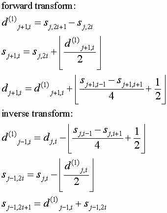
I have implemented three integer to integer Lifting Scheme wavelet transforms. This are listed below, along with the equations for the forward and inverse transform. One of the elegant things about the wavelet Lifting Scheme is that the inverse transform is the mirror of the forward transform, with the + and - operators interchanged.
-
An integer version of the Lifting Scheme version of the Haar transform. In image processing this is known as the S transform.
 ,
, -
An integer version of the linear interpolation wavelet transform. The linear interpolation transform "predicts" that an odd element will be on a line between its two even neighbors. The difference between this "prediction" and the actual value becomes the wavelet coefficient (sometimes called the detail coefficient). The scaling function is simply the average of the original even and odd elements.
 ,
, -
An integer version of the Cohen-Daubechies-Feauveau (3,1) wavelet transform. This is sometimes referred to as the TS transform in the image processing literature.
 ,
,
The wavelet lifting scheme is discussed on the related web page Basic Lifting Scheme Wavelets. The equations above correspond to lifting scheme steps.
The notation used here is based on the notation in [2], so I'll briefly try to explain it.
The forward wavelet transform takes N elements in step j and calculates N/2 detail coefficients (shown as d above) and N/2 scaled values (shown as s above). The scaled values become the input for the next step of the wavelet transform (which is why these values are shown with the subscript j+1). In the next step, Nj+1 = Nj/2.
The inverse wavelet transform in step j rebuilds the sj-1,i and sj-1,i+1 (even and odd elements) from the dj and sj values.
References:
-
State of the Art Lossless Image Compression Algorithms by S. Sahni, B.C. Vemuri, F. Chen, C. Kapoor, C. Leonard, and J. Fitzsimmons, October 30, 1997
-
Wavelet Transforms that Map Integers to Integers by A.R. Calderbank, Ingrid Daugbechies, Wim Sweldens, and Boon-Lock Yeo, 1996