Rendering Massive Terrains using Chunked Level of

Detail Control

DRAFT

Thatcher Ulrich
Oddworld Inhabitants
tu@tulrich.com

Revised 14 April 2002

Source of information: http://tulrich.com/geekstuff/sig-notes.pdf

Figure 1: The first three levels of a Chunked LOD tree

1 Introduction

Outdoor terrain rendering is important for a large class of game and simulation applications. Hardware and algorithms continue to improve rapidly, which enhances our ability to render realistic terrains. The shift in recent years in consumer hardware from CPU bound graphics pipelines to high speed special purpose graphics processing units (GPUs) has drastically changed the tradeoffs in geometric level of detail (LOD) terrain rendering algorithms. These new tradeoffs have sparked the development of GPU-oriented aggregated LOD algorithms. Furthermore, the increased quantity and detail of the data sets we can render has raised the demand for data to feed to our renderers, and highlighted the importance of handling data sets which do not fit in RAM (out-of-core data sets).

Meanwhile, advances in shading and image quality in general have raised end-us expectations for image quality and lowered their tolerance for visual artifacts. These notes briefly review the problems of constructing an ideal terrain renderer, mention the most popular and successful existing algorithms, and then present Chunked LOD, a novel approach to aggregated LOD. Chunked LOD has a number of practical advantages over previous schemes, including ease of texturing, low CPU load and simple handling of out-of-core data sets.

2 The Ideal Terrain Renderer

The ideal terrain renderer would let the viewer stand at the summit of a tall mountain and see the surrounding countryside in perfect detail, from the trees on a distant ridge line to the pebbles at the viewer's feet. The viewer would freely move around the scene, walking through dense forests or flying rapidly through the air directly to some distant spot, where both the local surroundings and distant vistas would always be perfectly detailed to within the limits of the display. The place represented by the ideal terrain renderer could be a faithful model of part of the real world, or some imaginary locale, but in either case should be visually rich and interesting. At no point should the viewer be aware of any distracting artifacts arising from the shuffling of data or reorganizing of geometry within the renderer itself.

Unfortunately we are not yet able to make the ideal terrain renderer. In the meantime we would like to get as close as we can with the technology we do have, and it turns out that we can do quite well in some respects.

3 Heightfields and LOD

In these notes I am going to restrict my focus to heightfield rendering. Heightfield rendering is a smaller, but important, sub problem of constructing the ideal terrain renderer described above. Heightfields are not strictly necessary, and in fact are not sufficient in themselves for ideal terrain rendering, especially when the viewer gets close to the ground. But the heightfield format is a very useful approximation. It embodies a basic method of compression and a framework for organizing data and textures. There are also many existing heightfield algorithms, tools and data sets to build on.

There are a number of good solutions for heightfield level of detail (LOD) rendering which effectively reduce the number of triangles which need to be rendered, at the expense of doing some run-time meshing calculations. Probably the most popular approach is to use a restricted quadtree or binary-triangle tree. The most commonly cited papers are [7] [4] and [10], and they all work quite well, with a number of publicly available implementations. They generally involve some preprocessing and a little extra per-vertex error data over and above a standard heightfield. Another important set of LOD algorithms is derived from Hoppe's Progressive Meshes [5].

Progressive Meshes focus on general meshes rather than heightfields in particular, which results in somewhat different trade offs, but have been successfully applied to heightfields.

4 Detail and visual richness

A major problem that soon becomes apparent when you experiment with demos of the systems is the limited amount of detail present in the data. The frame rate is high, the mesh is seamless, but when you get close to the ground things get very blurry and smoothed out, and when you go high into the air you eventually see the edge of the data.

The difficulty here is that we just cannot store enough heightfield and texture data in RAM to get the detail we want over large areas. One typical solution is to store a very large data set out-of-core — on a local disk, or on a networked server — and page in only the data required for a particular view. Several of the LOD references, particularly [8], address the issue of out-of-core storage, but high quality consumer-level solutions are still lacking.

From a game programming perspective, there are also some alternative approaches to making huge terrains that do not involve out-of-core storage at all. One approach is to use adaptive detail, using a multiresolution representation so that 'important' areas of the terrain have lots of data, while less important areas use very little data. This can nicely solve some practical problems, but is not a general solution, as it puts detail and richness in the virtual world in conflict with freedom of movement for the viewer.

Another approach is to create procedural detail on the fly as it is needed. This is a very powerful technique, but has significant limitations. The difficulties here include processing time — beautiful and interesting terrains can be generated procedurally with packages like Bryce or Mojoworld, but achieving such high quality takes a lot of processing time, and must typically be done in a preprocessing stage. Another open problem is making procedural terrains controllable enough so that game designers and artists can achieve the specific results they want.

In these notes I am focusing mainly on rendering large, static out-of-core data sets, since the trade-offs are less application-dependent than with procedural or adaptive detail. Nevertheless, I don't want to minimize the importance of these other approaches. Real applications usually need to implement some combination of approaches to achieve good results.

5 Level of Detail and Perspective

Because of perspective, when we stand on a terrain in the real world and look out over a vista, our view covers a wide scale of geometric detail. We can resolve 1mm details in the pebbles at our feet, but in the far distance, a 100m cliff on the side of a mountain may be the smallest thing we can resolve. That is a factor 10⁵ in geometric size difference, due entirely to perspective. Exploiting this effect is central to scalable terrain LOD control.

The good existing schemes generally can guarantee that a mesh is rendered within some maximum screen-space error tolerance, “Tau”, while taking advantage of the perspective transform to render fewer and fewer triangles as distance from the viewer increases.

6 Texturing

Texture mapping sometimes gets short shrift in the terrain LOD literature, but in practice it is critical for good visual results. Shading is a key indicator of geometric shape and detail, but it is impractical to achieve quality pixel-level fine detail using geometry only. Among other things, graphics hardware is much better at antialiasing minified textures than it is at antialiasing sub-pixel vertex shading. Textures are also relatively compact for this purpose.

Like our geometry, we would like our texture mapping to be scalable over a 10⁵ range of detail levels. Fortunately, it is not as difficult to seamlessly match up texture edges as it is to match up geometry edges. Quadtree tiling is a straightforward, fully scalable solution to the problem [12]. A serious difficulty lies in integrating tiled texturing with scalable geometric LOD. We cannot draw more than one texture map per triangle, and for efficiency we would like to draw many triangles with the same texture. At the same time for image quality and to avoid LOD artifacts, we would like to maintain a texture density of least one texel per visible pixel on screen. We need our geometric LOD solution to be compatible with those constraints.

7 Pre-GPU LOD Algorithm

In these notes, I am using the term GPU to refer to a class of low cost high speed specialized vertex processing hardware, such as the NVIDIA GeForce, ATI Radeon and Sony PlayStation 2. This class of hardware incorporates one or more floating point transformation units in addition to the integer pixel rasterization hardware common in the previous generation of consumer graphics hardware. The floating point vertex processing done by these high speed GPUs had previously been the responsibility of the general purpose CPU, greatly limiting triangle throughput.

Prior to the widespread adoption of GPUs, LOD algorithms for game applications focused on minimizing the number of triangles drawn, at the expense of a limited amount of extra CPU processing. Various published algorithms for this, such as Lindstrom-Koller CLOD [7], ROAM [4] and Progressive Meshes [5] were adopted and adapted to become a useful component in the game programmer's toolbox. The additional processing necessary to compute scalable LOD meshes was typically more than made up for by the time saved by transforming fewer vertices for rendering.

Post-GPU LOD Algorithm

With the advent of GPUs, consumer hardware saw maximum triangle rendering rates skyrocket. CPU involvement in rendering could be limited to merely pointing the GPU at a section memory containing the vertices of a model to render. Developers interested in producing top quality graphics for games often focus on either brute force all-GPU methods (i.e. no continuous LOD), or approaches with very low CPU overhead, like View Independent Progressive Meshes [1][11].

Unfortunately, those algorithms are not view dependent, and it is not obvious how t scale these methods to terrain data sets with a seamless 10⁵ ratio between near and far detail. Likewise, reorganizing the continuous LOD approaches to achieve low CPU overhead presents many difficulties

Chunked LOD

Nevertheless, an efficient, hardware-friendly continuous LOD algorithm is highly desirable and there are a number of published approaches that have achieved success at solving the core geometric LOD problem. These approaches commonly exploit two strategies individually or in combination:

1) Apply a view-dependent LOD algorithm to aggregates of primitives, not individual primitives.

2)Cache the results of a vertex-level LOD algorithm to reuse them for similar viewpoints

Various approaches are detailed in [3], [1], [2], [6] and [9]. The permutations are too numerous to summarize here, so I refer you to the individual descriptions.

Chunked LOD is yet another variation on strategy 1 above. Like some of the other aggregated approaches, it achieves low CPU overhead and high triangle throughput However, it uniquely combines several other important advantages:

-Efficient use of triangles within aggregates

-Texture LOD integrated with geometry LOD.

-Easy to integrate with out-of-core storage

-Efficient, smooth vertex morphing; no vertex pops

-Low CPU load, even when viewpoint moves rapidly

The negative characteristics include:

- Non-trivial preprocessing required.

- Data set must be static

- Uses more triangles than a primitive level algorithm, for the same screen-space error

- Some data size overhead, depending on lossiness of preprocessing.

The general approach to Chunked LOD is laid out in [1], although in the context of using view-independent progressive meshes for the chunks. [2] covers the usage of quadtrees of meshes, with morphing of static meshes to avoid popping artifacts, but relies on regular grid subdivision within each mesh, and is not easily amenable to out-ofcore paging.

The method presented in these notes builds on those ideas and works out a number of important details.

At the heart of the method is a tree of static, largely independent preprocessed meshes The tree and its component meshes (the "chunks") are generated in a preprocessing step, based on a high-detail reference mesh. Each chunk is just a static mesh primitive that can be rendered with a single glDrawElements() or DrawPrimitive() call, plus an additional fast morphing pass. The chunk at the root of the tree is a low-detail representation of the entire object. The child chunks of the root node split the object into several pieces, and each piece independently represents its portion of the object with a higher level of detail than the parent.

This relationship is recursive down to some arbitrary depth. Each chunk has a bounding volume associated with it, as well as a maximum geometric error, “S”. “S” represents the maximum geometric deviation of a chunk (in object space) from the portion of the underlying full-detail mesh it represents.

For simplicity's sake, I assign the same “S” to all the meshes at a particular level in the chunk tree. Furthermore, I compute “S” such that:

Where L is the level in the tree. For example, if the root node of the tree is a single mesh that represents the object with at most 16 units of deviation from the original full-detail mesh (“S”(0) = 16) then the second level contains several chunks that each represent a piece of the object with at most 8 units of deviation from the full-detail mesh (“S”(l) = 8). At the fifth level down the tree, the chunks each represent a small piece of the object, with only 1 unit of deviation (“S” (4) = 1).

When we apply this splitting scheme to a heightfield, the simplest approach is to organize the tree as a quadtree of heightfield sub-squares (see figure 1). This will also prove convenient when we consider texture mapping.

10 View dependent rendering

At run time, to render the object, we simply choose the chunks that represent each part of the object to meet our desired visual fidelity. Since we have a bounding volume for each chunk, and a maximum geometric error for the vertices within a chunk, we can use a standard LOD formula for conservatively determining the maximum screen-space vertex error, “p”, for a chunk:

Where “S” is the maximum geometric error of a chunk, D is the distance from the viewpoint to the closest point on the chunk's bounding volume, and K is a perspective scaling factor that takes into account the viewport size and field-of-view, and is computed by:

Note that, as is common in the LOD literature, “p” is measured at the center of the viewport, which is slightly liberal but reasonable. From the standpoint of efficiency, there is no compelling reason not to use a more precise, more expensive screen-space error metric; unlike per-vertex LOD algorithms, the view metric typically only needs to be evaluated on the order of a couple hundred times per frame. Nevertheless, this simplified metric is very effective in practice, and because it is independent of view direction, the LOD mesh stays absolutely stable when the viewer rotates in place.

A simple way to evaluate our LOD tree and render the chunked model is to traverse the tree, starting at the root. We start out by choosing a value for our maximum tolerable screen-space error, “r”. Then, given a chunk, we can use equation 1 to determine whether the screen-space error is acceptable. If it is, then we render the chunk and do not recurse to the children. If it is not acceptable, then we recurse to the child nodes. Pseudocode:

There are two big problems with the above algorithm:

1. Neighboring chunks at different LODs will have cracks where they meet.

2. When the viewpoint approaches a chunk, the chunk will split into several child chunks, and the mesh shape will pop suddenly. Because many vertices are popping at the same time, this is much more objectionable than the single vertex popping in common ROAM or PM-based implementations

Effective solutions to both problems follow.

11 Crack filling

There are several ways to fix the cracks between meshes. One obvious approach is to always decimate the edges of chunks to some globally constant geometric error, regardless of the chunk's actual “S”. Unfortunately this severely limits scalability. A better variation on this is to restrict the relationship of neighboring chunks, and always decimate to a regular scale-relative pattern at the edge [6] [9], although this is not optimal either.

Figure 2: Using a flange to fill a crack. The white triangle on the left is a crack between two meshes. A flange (marked in black) is added to one of the meshes; it extends into the other mesh and interpenetrates, covering the crack.

Another method is to add 'flanges' around each chunk, so the meshes interpenetrate slightly. This should usually work well, but avoiding artifacts gets a little messy. In particular, choosing the angle and size of the flanges is somewhat ad hoc and depends on the precise geometry of the neighbor. Proper texturing of the flanges is slightly complicated as well.

Yet another approach is to join the chunks with special meshes. These can be generated using a two- or three-level scheme, by joining the edge of the interior of a chunk with the edge of the interior of the neighboring chunk. Unfortunately this can be complicated, as it requires the definition of an explicit interior to each chunk, and the relationship between the special meshes and screen-space error is not clear.

Figure 3: Using a ribbon to fill a crack. A vertical ribbon (marked in black) has been added which perfectly fills the crack by sharing the vertices adjacent to the crack.

A somewhat simpler variation on the above is to generate a vertical "ribbon" mesh, to join the edges between chunks. This works solely off the edge vertices of the chunk and is visually very effective. Note that the vertical ribbon meshes stay within the bounds of a chunk, and can be shaded using the associated chunk's texture. Clearly this results in vertical texture stretching over the ribbon, but note that the ribbon is always smaller than “r” pixels on screen. For reasonable values of “r”, the stretching is practically undetectable. This method is still somewhat complex, especially when combined with the anti-popping.

Figure 4: Using a skirt to fill a crack. A vertical skirt (marked in black) has been added t one of the chunks, to fill the crack without actually extending into the other chunk.

solution described below, because it depends closely on the precise geometry of the edges of both chunks.

The crack filling method I prefer combines the virtues of flanges and ribbons. The idea is to simply create a vertical "skirt" around the perimeter of each chunk. The top of the skirt matches the chunk edge, while the bottom does not match anything in particular. The requirement of the bottom edge of the skirt is that it extends below the full LOD mesh at the edge, as well as below any possible simplifications of the edge. Also, we would like the skirt to be as short as possible to conserve fill rate. Like flanges, the skirts are self-contained by a chunk and are composed of simple static triangles. Like ribbons, skirts do not extend into the interior of any neighboring node and may be textured by simply using the chunk's existing texture.

Figure 5: Texture stretching on vertical skirt (in highlighted area), ”R” has been set to 35 to illustrate stretching. For more normal values of “R” (usually < 5), texture stretch is very hard to see.

12 Avoiding Pops

As mentioned above, we can hide the ugly visual transition when a chunk splits into it s child chunks, or when child chunks merge into a parent chunk. The solution involves applying a small (possibly 0) morph to the vertical coordinate of each vertex in a chunk mesh, using a single uniform morph parameter over the whole chunk. The morph target is computed as follows: for each vertex in a chunk, its morph target has the same horizontal coordinates. The vertical coordinate is computed by sampling the height of the parent chunk and the known horizontal coordinates.

At rendering time, we will compute a chunk's morph parameter, ensuring that the morph parameter is always 0 when the chunk is about to split, and 1 when the chunk is about to merge. This guarantees that the shape of a chunk at the distance where a split occurs is identical to the shape of the chunk chunks at an infinitesimally closer distance after the chunk has split.

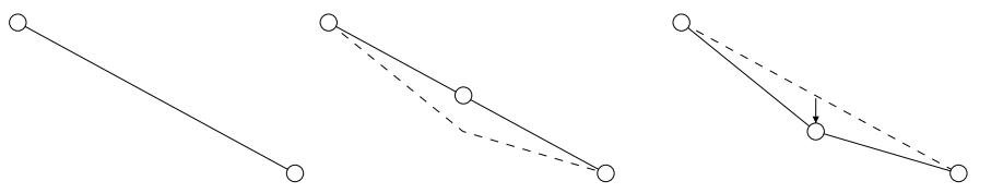
Figure 6: A 2D illustration of pop avoidance. On the left is a line with two vertices representing part of a low-detail chunk. In the middle, it has been replaced by a line with three vertices, representing a higher detail child chunk. The dashed line shows the desired true shape of the chunk, but the middle vertex has been morphed to match the low-detail parent chunk. On the right, the middle vertex has morphed into its desired position.

Rearranging our error metric, we can directly compute such a morph parameter given the distance to the chunk.

This formula produces t_morph = 0 at the distance at which the chunk's parent splits (because the parent's ”S” is double the child's “S”, and the parent's bounding volume contains the child). It produces t_morph = 1 exactly at the point at which the chunk itself will split. It linearly interpolates tmorph in between those distances, as the viewer gets close to the chunk.

This avoids the visual artifact caused by many simultaneous vertex pops. In fact, it completely eliminates all vertex pops throughout the tree, replacing them instead with a subtle morph. The actual LOD transition when a chunk is split into its children is completely undetectable to the viewer. Note that when using our simple error metric, morphing is based entirely on viewpoint distance, which has the nice property that the mesh only morphs when the viewpoint moves. This further reduces the noticeability of morphing.

The data cost of this morphing scheme is the addition of either a morph target or a morph delta per vertex. A morph delta may be preferred because it can be quantized into very few bits. The morph delta will always be smaller than “r” pixels on-screen, so the quantization error in screen space is less than “r”/(2^N) where N is the number of bits allocated for the morph delta.

There is also the on-the-fly processing required to adjust the vertex data. Because the morph parameter is uniform over an entire chunk, and the vertex data for a chunk is just a simple linear array, even a naive CPU implementation is fast enough to feed a hungry GPU pipeline. For reduced CPU load, a straightforward vertex program (vertex shader) may be used instead.

13 Texturing

Texturing for this LOD scheme is very simple — at preprocessing time, we just provide a static texture for each static chunk. Given knowledge of the screen-space error metric used at run-time, and an upper bound on the runtime value of “r”, our preprocessor can guarantee that the projected texel size at run time will not exceed 1 texel per pixel. The math goes like this: Let D_min be the minimum geometric distance at which a chunk will be displayed. From formula 1, we have:

where T_s is the projected size of a texel on-screen, and T_g is the geometric size of a texel for the texture of a chunk. Solving for T_g ,and substituting 1 for T_s we get:

We can use this formula for T_g to force a minimum texture resolution for each chunk a preprocessing time. Note that if we are using a simple 2D mapping to assign texture coordinates, this formula does not account for texture stretch due to steeply sloping surfaces. We can optionally compute texture stretch as well, based on the known chunk geometry, and take it into account.

14 Compression

The chunk hierarchy, crack-filling meshes, and vertex morphing information impose a substantial size overhead on the storage required for a chunk tree, compared to a simple static mesh of the same object or a heightfield representation. However, there are a couple of significant factors which help offset this overhead.

The preprocessing step in Chunked LOD completely discards vertices which are not necessary to approximate the mesh to within the minimum value of “S” (at the highest LOD in the tree). This acts as a form of lossy compression on the original heightfield. Flat areas are heavily decimated. For typical real-world DEM models, the compression is usually significant, even for very modest degradation in the heightfield shape.

Another potentially useful property of Chunked LOD is that the vertices in individual chunks are spatially localized. The chunks vary in size in world coordinates, but because of the LOD algorithm, stay within restricted bounds in screen coordinates. If the vertices in a chunk are compressed using a simple quantization scheme, the quantization errors will be bounded in screen space. This fails to hold true when zooming in on the finest chunk level; however, for reasonable tree depths (e.g. up to 8 levels) 8 bits of precision should be enough for even large data sets.

Taking into account all overhead, the reference implementation of the chunk preprocessor produces chunk data files (geometry only, no textures) ranging from around 25 to 35 bytes per unique output vertex, depending on the data and the preprocessing parameters. For typical DEM data and very modest lossy compression, this may correspond to around 5 to 7 bytes per heightfield sample in the input data. These figures do not yet reflect the aggressive quantization compression possibilities mentioned above, so a realistic minimum data size for Chunked LOD will be smaller.

15 Paging out-of-core chunks

All mesh and texture data for each chunk is self-contained. This makes it fairly easy to page in detail on demand. The general approach is to run a separate thread which is responsible for loading chunk data. The render pseudocode is modified as follows:

Additionally the loading thread should free the storage used by a node's geometry data when it has not been used for some time

16 Implementation

I have made a free, public domain reference implementation of the Chunked LOD algorithm presented here. It runs on Windows and Linux, and should be adaptable to other platforms. I encourage anyone who is interested to use and adapt the code for any purpose. Credit, bug fixes and improvements are always appreciated, of course, but there are no restrictions whatsoever on how the code may be used.

17 Acknowledgments

Thanks are due to Oddworld Inhabitants for supporting the presentation of this work and fostering a work environment where personal research is encouraged. Sean Barrett, Charles Bloom, Jon Blow, Mark Duchaineau, Tom Forsyth, Josh Levenberg and Aaron Pfeiffer for comments, criticism and ideas. Thierry BergerPerrin and Mike Shaver for providing additional code, bug fixes, and Linux build improvements. John Ratcliff, Peter Lindstrom, Ben Discoe, Ken Musgrave, the University of Washington and the US Geological Survey for providing sample data.

References

[1] C. Bloom. View independent progressive meshes VIPM). World wide web, Jun 000. http://www.cbloom.com/3d/techdocs/vipm.txt

[2] D. Cline and P. K. Egbert. Terrain decimation through quadtree morphing. IEEE Transactions o n Visualization and Computer Graphics, 7(l):62-69, Jan-Mar 2001

[3] W. H. de Boer. Fast terrain rendering using geometrical MIP mapping. World wide web, Oct 2000. http://www.flipcodecom/tutorials/tutgeomipmapsshtml

[4] M. A. Duchaineau, M. Wolinsky, D. E. Sigeti, M. C. Miller, C. Aldrich, and M. B. Mineev-Weinstein. ROAMing terrain: Realtime optimally adapting meshes. In IEEE Visualization '97, pages 8188, 1997.

[5] H. Hoppe. Progressive meshes. In Proceedings SIGGRAPH 96, pages 99108. ACM 1996.

[6] J. Levenberg. Fast view-dependent level-of-detail rendering using cached geometry. Forthcoming, Mar 2002.