Hierarchical clustering with CUDA/GPU
Ŕâňîđű: Dar-Jen Chang, Mehmed Kantardzic, Ming Ouyang
Čńňî÷íčę: http://www.cs.stevens.edu/...
Abstract
Graphics processing units (GPUs) are powerful computational devices tailored towards the needs of the 3-D gaming industry for high-performance, real-time graphics engines. Nvidia Corporation provides a programming language called CUDA for general-purpose GPU programming. Hierarchical clustering is a common method used to determine clusters of similar data points in multidimensional spaces; if there are n data points, it can be computed in O(n2) to O(n2log(n)) sequential time, depending on the distance metrics employed. The present work explores parallel computation of hierarchical clustering with CUDA/GPU, and obtains an overall speed-up of up to 48 times over sequential computation with an Intel Pentium CPU.
Introduction
Graphics processing units (GPUs) on commodity video cards have evolved into powerful computational devices tailored towards the needs of the 3-D gaming industry for high-performance, real-time graphics engines. In the past, software development on GPUs has been geared exclusively towards graphics through the use of languages such as OpenGL shading language and Direct3D high-level shader language. In 2006, Nvidia Corporation released a new generation of GPUs designed for general purpose use. These G80 series GPUs provide up to 128 stream processors and support 12,288 active threads. This new architecture facilitates efficient general purpose computing on GPUs (GPGPUs). In 2007, Nvidia Corporation released an extended C language for GPU programming called CUDA [13], short for Compute Unified Device Architecture. Using CUDA, innovative dataparallel algorithms can be implemented in general computing terms to solve many important and non-graphics applications such as database searching and sorting, medical imaging, protein folding, and fluid dynamics simulation.
Hierarchical clustering [10] is commonly used in exploratory data analysis. It determines clusters of similar data points in multidimensional spaces. At the beginning of hierarchical clustering, each data point is considered a separate cluster. The two clusters that are closest according to some metric are joined to form a new cluster. This process is repeated till all of the points belong to one cluster. The final hierarchical cluster structure is called a dendrogram. Two kinds of distance metrics are employed in the process. The first kind determines the distances between two individual data points and will be referred to as pairwise distances henceforth. Some common choices are Euclidean distance, Manhattan distance, and Pearson correlation coefficient. The second kind of distance metrics concerns the distances between clusters consisting of multiple data points. When there are multiple pairwise distances between two clusters, what is the “distance” between the clusters? Some common choices are single link (the minimum of pairwise distances), complete link (the maximum of pairwise distances), and average link (the average of pairwise distances).
Hierarchical clustering is a well established method in data analysis. In recent years it is widely used in bioinformatics. The DNA microarray technology [1] assays messenger RNA (mRNA) abundance of cell samples. A DNA microarray simultaneously measures the mRNA levels of thousands to tens of thousands of genes in one experiment. Scientists usually conduct studies consisting of dozens to a couple hundreds of microarray experiments. The data are collected in a matrix where the rows correspond to the genes, the columns correspond to the experimental conditions, and each entry in the matrix is the abundance of the gene under the particular condition. During the exploratory phase of data analysis, scientists often apply hierarchical clustering on the genes, under the assumption that genes with similar regulatory pathways or with similar biological functions will cluster together. The popularity of hierarchical clustering in DNA microarray data analysis is probably due to the early introduction of Michael Eisen’s Cluster software [7]. Other clustering methods, such as k-means [10] and self-organizing maps [18] are also in use, albeit with less frequency.
A common feature of these clustering algorithms is dataparallelism, or single instruction multiple data (SIMD) computation. That is, the same calculation is performed over numerous pieces of computationally independent data. There are several CUDA implementations of k-means that can be easily located on the world wide web. Unfortunately, it is difficult to delineate the development chronology and authorship because many authors did not pursue formal publication. For hierarchical clustering, Zhang and Zhang [20] used a shader language and achieved 2-4 times of speedup compared to a CPU implementation. An important operation in hierarchical clustering is to calculate all pairwise distances. Chang et al. [2] used CUDA/GPU to compute pairwise Euclidean distance and achieved 20 to 44 times of speed-up over CPU, and the method was further extended to Manhattan distance and Pearson correlation coefficient with 40 to 90 and 28 to 38 times of speed-up, respectively [3].
In the present work, a CUDA/GPU implementation of single linkage is described. Incorporating prior work on pairwise distances, this is the first complete implementation of hierarchical clustering on the CUDA/GPU platform. In Section 2, CPU and CUDA/GPU implementations of single linkage are presented. In Section 3, computational results are presented, which show an overall speed-up of up to 48 times over sequential computation with CPU. In Section 4, possible improvements and future work are discussed. It is important to note that there are many publications in the literature on hierarchical clustering using either theoretical models of parallel computation [4], [12], [14], [16], [19] or expensive hardware [5], [6]. The focus of the present work is to perform the task using commodity hardware in a desktop computing environment.
Data and Methods
Data
In a cDNA microarray experiment [1], a microarray chip is hybridized to the mixture of a control sample and a treated sample. There are thousands to tens of thousands spots on the chip. Each spot typically yields two 16-bit integers; they are the abundance indices of the gene in the control and treated samples. A common practice in microarray data processing is to take the base-2 logarithm of the ratio of treatment over control. Thus a positive number indicates up-regulation of the gene in the treated sample, a negative number indicates down-regulation, and a zero means there is no change. Microarray data are known to be very noisy, despite various preprocessing, normalization, and transformation [15]. Therefore, although many software tools generate double-precision numbers, single-precision (4 bytes, or float in C) is more than adequate to store these resulting numbers.
Let n be the number of genes and let m be the number of experimental conditions. In data mining, n is known as the number of objects and m is the number of features. The data used in the present study were retrieved from Stanford Microarray Database [17]. In order to compare the performance of program code on data with different sizes, n takes a value from 4,096, 8,192, 12,288, and 16,384, and m takes a value from 16, 32, 64, and 128. These numbers represent typical ranges of microarray data clustering. For example, the budding yeast (Saccharomyces cerevisiae) genome has 6,300 genes and the human genome has 20,000 genes. In most experimental conditions, the majority of the genes will not be perturbed by the treatments. Thus researchers often select a subset of the genes for cluster analysis. The largest numbers of genes and experiments (16,384 and 128, respectively) represent realistic scenarios of microarray data analysis.
CPU C code
void cpuRho(float * out, float * in, int n, int m){
	int i, j, k;
	float x, y, a1, a2, a3, a4, a5;
	float avgX, avgY, varX, varY, cov, rho;
	for(i=0;i<n;i++){
		out[i * n + i] = 1.0;
		for(j=i+1;j<n;j++){
			a1 = a2 = a3 = a4 = a5 = 0.0;
			for(k=0;k<m;k++){
				x = in[i * m+k], y = in[j * m+k];
				a1 += x, a2 += y;
				a3 += x * x, a4 += y * y, a5 += x * y;
			}
			avgX = a1/m, avgY = a2/m;
			varX = (a3 - avgX * avgX * m)/(m-1);
			varY = (a4 - avgY * avgY * m)/(m-1);
			cov = (a5 - avgX * avgY * m)/(m-1);
			rho = cov/sqrtf(varX * varY);
			out[i * n + j] = rho;
		}
	}
}
Let us assume that the data are an n×m matrix M, stored in a float array called in in row-major order. The code needs compute an n×n matrix of pairwise distances (Euclidean distance, Manhattan distance, or Pearson correlation coefficient), to be stored in a float array called out in row-major order. Because all these distance metrics are symmetric, only the upper triangle of out needs to be computed. Euclidean distance and Manhattan distance are straightforward to compute. Pearson correlation coefficient (ρ) between rows i and j is defined as
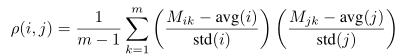 For each pair of i and j, three separate and sequentially executed for loops are needed if a straightforward implementation is employed: one loop to calculate avg(i) and avg(j), followed by another loop to calculate std(i) and std(j), and followed by the other loop to calculate Equation. However, it is undesirable to employ three separate loops sequentially processing a large array with modern paged memory management, for the loops may incur many page faults. Figure 1 has the CPU C code for pairwise Pearson correlation coefficient using one for loop (indexed by k) for each pair of i and j. The code in Figure 1 can be further improved for speed by moving the calculation of a1 and a3 from the innermost loop to the outermost one so that the computation for avg(i) and std(i) is not repeated for every value of j. However, it is thought that clarity in Figure 1 is more important than the fastest possible execution speed.
The sequential construction of single link hierarchical clustering has been described many times in the literature. There are n−1 iterations, and each iteration joins two nearest clusters. An iteration can be completed in O(n) time, based on the same agglomerative nearest neighbor (SANN) property [14]: if clusters A and B are agglomerated into cluster A+B, any cluster that had either A or B as its nearest neighbor now has A+B as its nearest neighbor.
The CUDA language
Nvidia Corporation has released a programming guide to the CUDA language [13], which is an extension of the C language [11]. Briefly, the Single Program Multiple Data (SPMD) code is written in a GPU kernel function, the data to be operated on are copied from CPU RAM to the video memory of the device, and the C program running on the CPU initiates the data-parallel computation via a kernel function call. A GPU kernel function contains the code that will be executed simultaneously by the GPU processors, and CUDA uses the function type qualifier __global__ to declare that a function is a GPU kernel function. For example,
__global__ void gpuRho(...){
...
}
tells the CUDA compiler nvcc that gpuRho is to be executed
by the GPU.
The CUDA language supports a large number of threads. The threads are organized into blocks, where there may be up to 512 threads in each block. The blocks are further organized into a grid of up to (2^16-1)×(2^16-1) blocks. CUDA offers one- and two- dimensional grids and one-, two-, and three-dimensional blocks of threads. For example, let numRows be the number of rows of the data matrix, and the size of the matrix of pairwise distances is numRows x numRows. The code
dim3 block(16,16);
dim3 grid(numRows/16, numRows/16);
declares that there are 256 threads in a block (organized as a 16 by 16 square), and the blocks are arranged in a numRows/16 by numRows/16 grid. It is assumed that numRows is a multiple of 16. If it is not the case, one can add additional entries to the data matrix to make it so, and trim the pairwise distance matrix later on to remove the additional entries. The GPU device provides registers and local memory for each thread, a shared memory for each block, and a global memory for the entire grid of blocks of threads. Although all threads execute the same GPU kernel function, a thread is aware of its own identity through its block and thread indices, and thus a thread can be assigned a specific portion of the data on which it can perform computation. For example, a thread can locate its own position among the blocks and the threads using the following code:
int bx = blockIdx.x, by = blockIdx.y;
int tx = threadIdx.x, ty = threadIdx.y;
Often times the threads of the same block need to coordinate their computation. CUDA provides the function __syncthreads() that serves as a barrier. A thread is blocked from further execution if it finishes its work earlier than the rest, and the threads in the same block are released after all threads have reached the barrier. CUDA provides function calls to allocate memory on the GPU device, and to copy data from CPU RAM to the device memory and vice versa. Typical code looks like the following:
cudaMalloc((void ** )&gpuInput, inSze);
cudaMemcpy(gpuInput, input, inSize,
cudaMemcpyHostToDevice);
Then from the C code that is executed by the CPU, one may initiate the execution of the grid of blocks of threads on the GPU as follows:
gpuPdist<<<grid, block>>>(gpuOutput, gpuInput, otherParameters);
After the GPU kernel function exits, the results may be copied from the device memory back to CPU RAM. The shared memory for a block of threads is fast, yet it is limited in size. One strategy to attain high performance is for the threads in the same block to collaborate on loading data that they all need from the global memory to the shared memory. The shared memory is further partitioned into banks. The threads in the same block may access different banks simultaneously, yet a memory bank conflict will serialize the threads involved in the conflict. Thus another strategy for high performance is to avoid bank conflicts as much as possible.
CUDA/GPU code
The CUDA code for pairwise Pearson correlation coefficient is presented. The code for Euclidean distance or Manhattan distance is similar yet simpler than Pearson correlation. The data array in is n×m in row-major order of n genes and m microarray experiments, and an n×n matrix out of pairwise (gene-gene) distances will be computed. Figure 2 illustrates the idea of the CUDA algorithm. Let us assume that a thread needs to calculate the entry indexed by (i,j) in the matrix out where i is 16*by
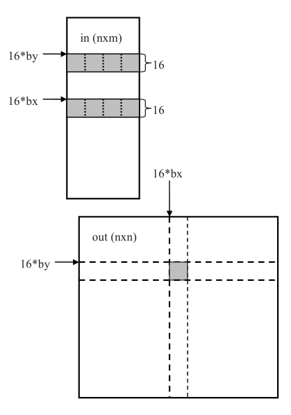 and j is 16*bx. Row 16*by of the matrix in is first copied to shared memory for fast access. While the copy of row 16*by is in shared memory, those threads that are responsible for entries (i,j+1),(i,j+2),...,(i,j+15) of the matrix out can all use the same copy for fast memory access. Similarly, after row j of the matrix in is copied to shared memory, the threads that are responsible for entries (i,j),(i+1,j),...,(i+15,j) can use the same copy. Thus it is advantageous to have square blocks of threads that share the data in the shared memory. Blocks of 16 by 16 threads are used because CUDA limits the maximum number of threads in a block to 512.
Next wrapper has the CUDA/GPU code that computes the pairwise Pearson correlation coefficient. The algorithm uses one thread for one entry in out. Thus there are n 2 threads. The threads are organized into 16×16 two-dimensional blocks, and the blocks are organized into an n/16×n/16 two-dimensional grid. A thread orients itself through its block and thread indices in the following way:
int bx = blockIdx.x, by = blockIdx.y;
int tx = threadIdx.x, ty = threadIdx.y;
__global__ void gpuRho(float* out, float * in, int n, int m){
	__shared__ float Xs[16][16];
	__shared__ float Ys[16][16];
	int bx = blockIdx.x, by = blockIdx.y;
	int tx = threadIdx.x, ty = threadIdx.y;
	int xBegin = bx*16*m;
	int yBegin = by*16*m;
	int yEnd = yBegin + m - 1;
	int x, y, k, o;
	float a1, a2, a3, a4, a5;
	float avgX, avgY, varX, varY, cov, rho;
	a1 = a2 = a3 = a4 = a5 = 0.0;
	for(y=yBegin,x=xBegin;y<=yEnd;y+=16,x+=16){
		Ys[ty][tx] = in[y + ty * m + tx];
		Xs[tx][ty] = in[x + ty * m + tx];
		// *** note the transpose of Xs
		__syncthreads();
		for(k=0;k<16;k++){
			a1 += Xs[k][tx], a2 += Ys[ty][k];
			a3 += Xs[k][tx]*Xs[k][tx];
			a4 += Ys[ty][k]*Ys[ty][k];
			a5 += Xs[k][tx]*Ys[ty][k];
		}
		__syncthreads();
	}
	avgX = a1/m, avgY = a2/m;
	varX = (a3-avgX * avgX * m)/(m-1);
	varY = (a4-avgY * avgY * m)/(m-1);
	cov = (a5-avgX * avgY * m)/(m-1);
	rho = cov/sqrtf(varX * varY);
	o = by * 16 * n + ty * n + bx * 16 + tx;
	out[o] = rho;
}
With the above coordinate system, a thread is responsible to calculate the entry in the matrix out at row by * 16 + ty and column bx * 16 + tx, and it coordinates its calculation with the other 255 threads in its block in the following manner. During each iteration through the outer for loop, the 256 threads first load the two 16 by 16 sub-matrices of in anchored by the variables y and x at the corresponding upper left corners. These sub-matrices are aligned as depicted at past. After the threads are synchronized, each of them calculates and accumulates its own partial Pearson correlation coefficient in the variable s. Then the threads need to be synchronized again before proceeding to the next pair of 16 by 16 sub-matrices. A subtle yet very important point in the code is that the array Xs in the shared memory is transpose of its image in the matrix in. Through the transpose of Xs, the number of bank conflicts is reduced in the shared memory access by a factor of 16 and dramatically speed up the calculation.
Harris [8] described a time and work efficient CUDA/GPU algorithm for prefix sum (scan) that parallelized a seemingly sequential process. However, an important feature of parallel prefix sum is that the operator is associative, such as addition and multiplication. With associativity, the operations may be executed out of order, leading to time and work efficient parallelization. The link construction in hierarchical clustering is by nature a sequential process. As described in Section 2.2, there are n-1 iterations and each iteration joins two nearest clusters. The clusters that are joined in one iteration may impact the choices of those iterations that come afterwards. In other words, the linkage operations in hierarchical clustering are not associative. Therefore, the present study will sequentially construct the single linkage with n-1 iterations, and in each iteration, parallelize the work as much as possible.
Results
The performance comparisons are conducted with the following hardware and software setup. An Nvidia Tesla C870 GPU card is installed on a desktop computer with an Intel Pentium D 3GHz CPU and 2GB RAM. The Tesla C870 has a 128-processor core and 1.5GB RAM. The desktop operating system is Microsoft Windows XP Service Pack 3, and the C and CUDA code is compiled by Microsoft Visual Studio 2005, with optimization set for maximum speed (/O2) and floating point model set for “Strict.” The computation time is taken by the CUDA timer utility. As described in Section 2, DNA microarray data downloaded from Stanford Microarray Database [17] are used in the computational performance comparisons. The values of n (number of rows) are 4,096, 8,192, 12,288, and 16,384; the values of m (number of columns) are 16, 32, 64, and 128. The time to copy the input data to the GPU RAM is negligible: from less than 0.001 second for a 4096×16 float matrix to 0.008 second for a 16384×128 float matrix.
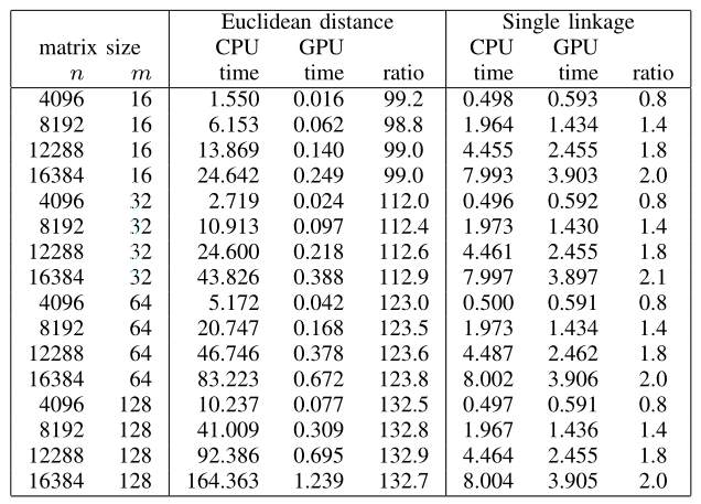
Table compares the CPU versus GPU computation time of pairwise Euclidean distance and single linkage. For pairwise distance, CUDA/GPU achieves 98-132 times speed-up for Euclidean distance, 174-210 times for Manhattan distance (data not shown), and 55-87 times for Pearson correlation coefficient (data not shown). For single linkage, CUDA/GPU achieves 0.8-2.1 times speed-up over CPU, regardless of the pairwise distance metrics. When CUDA/GPU pairwise distance computation time, single linkage computation time, and GPU RAM input/output time are all combined and compared to the CPU computation time, CUDA/GPU achieves overall 3.4-33 times speed-up for Euclidean distance, 5.8-48 times for Manhattan distance (data not shown), and 5.7-28 times for Pearson correlation coefficient (data not shown).
Discussion
The current trend in processor design is to pack multiple cores in a single chip. The challenge then is to fully utilize the numerous cores for parallel computation. General purpose computing on graphics processing units (GPGPUs) is emerging as a cost-effective way to boost the computation capability of desktop computers. With an Nvidia Tesla C870 GPU card (at a retail price of $1,000 US dollars or so) and carefully designed code, routine computation can be sped up by a factor of up to 48. In the past, this kind of improvement would require a Beowulf cluster at a much higher cost. In the present study, the benchmark goes up to 16,384 genes and 128 experimental conditions. These numbers are constrained by the amount of memory (1.5GB) on the GPU card, which puts a limit on the largest matrix that one may use. If 20 to 40 thousand genes are to be clustered, one needs to split the matrix of pairwise distances into pieces so that each piece fits the RAM of the GPU card. Furthermore, inter-GPU communication is needed to coordinate the computation and exchange the data. It is clear from Comparison Table that, as implemented in the present work, GPU is ill-suited for a strong sequential process such as linkage construction. GPU is at worst slower and at best no more than 2.1 times faster than CPU. It seems a lot of tedious coding for little gain. Nevertheless, it is still very useful to perform linkage with GPU for the following reason. The input data matrix from a DNA microarray study is relatively small (16384×128). However, the pairwise distance matrix is large (16384×16384). Should one be tempted to copy the pairwise distance matrix out of GPU for linkage by CPU, the copying time will eliminate a chunk of the GPU advantage. On the contrary, after linkage construction in GPU, the final data structure for the hierarchical clustering dendrogram is very small (16383×3; 16,383 being the number of internal nodes, the three numbers being the indices of the two children and their link distance) and can be copied to CPU RAM with negligible time. The DNA microarray experiments take a lot of time to conduct, from weeks to months. One may think that the CPU hierarchical clustering time of 3 minutes or so is already fast enough that any further speed-up is unnecessary. However, data analysts routinely apply statistical techniques, such as sub-sampling, boosting, and bagging, to explore the structures in the data. Additionally, computational scientists, during the development of new algorithms, will repeatedly apply clustering to perturbed data for validation. For these reasons, a fast hierarchical clustering tool on a commodity hardware will speed up the time to analyze new data and to develop new algorithms. Further work is needed to write CUDA/GPU code for other linkage methods, and it will benefit the reserach community if fast CUDA/GPU hierarchical clustering is made callable from popular data analysis platforms such as Matlab and R.
References
- Brown P, Botstein D. Exploring the new world of the genome with DNA microarrays. Nat Genet 1999, 21:33–7.
- Chang D, Jones NA, Li D, Ouyang M, Ragade RK. Compute pairwise Euclidean distances of data points with GPUs. Proceedings of the IASTED International Symposium on Computational Biology and Bioinformatics 2008, 278-283.
- Chang D, Desoky AH, Ouyang M, Rouchka EC. Compute pairwise Manhattan distance and Pearson correlation coefficient of data points with GPU. Proceedings of 10th ACIS International Conference on Software Engineering, Artificial Intelligence, Networking and Parallel/Distributed Computing (SNPD) 2009, in press.
- Dahlhaus E. Parallel algorithms for hierarchical clustering and applications to split decomposition and parity graph recognition. Journal of Algorithms (2000), 36:205-240.
- Dash M, Petrutiu S, Scheuermann P. Efficient parallel hierarchical clustering. Springer-Verlag LNCS (2004) 3149:363-371.
- Du Z, Lin F. A novel parallelization approach for hierarchical clustering. Parallel Computing 2005, 31:523-527.
- Eisen MB, Spellman PT, Brown PO, Botstein D. Cluster analysis and display of genome-wide expression patterns. Proc Natl Acad Sci U S A 1998, 95(25):14863–8.
- Harris M. Parallel prefix sum (scan) with CUDA. Nvidia Corporation 2007. http://developer.download.nvidia.com/compute/cuda/sdk/website/projects/scan/doc/scan.pdf
- Harris M. Optimizing parallel reduction in CUDA. Nvidia Corporation. http://developer.download.nvidia.com/compute/cuda/1 1/Website/projects/reduction/doc/reduction.pdf
- Hartigan JA. Clustering Algorithms, Wiley, New York, 1975.
- Kernighan BW, Ritchie DM. The C Programming Language, Second Edition, Prentice Hall, Inc., 1988.
- Li X. Parallel algorithms for hierarchical clustering and cluster validity. IEEE Transactions on Pattern Analysis and Machine Intelligence 1990, 12(11):1088-1092.
- Nvidia Corporation, NVIDIA CUDA Programming Guide, Version 2.0 June 7, 2008. http://developer.download.nvidia.com/compute/cuda/2.0-Beta2/docs/Programming Guide 2.0beta2.pdf
- Olson CF. Parallel algorithms for hierarchical clustering. Parallel Computing 1995, 21:1313-1325.
- Quackenbush J. Microarray data normalization and transformation. Nat Genet 2002, 32 Suppl:496–501.
- Rajasekaran S. Efficient parallel hierarchical clustering algorithms. IEEE Transactions on Parallel and Distributed Systems 2005, 16(6):497-502.
- Sherlock G, Hernandez-Boussard T, Kasarskis A, Binkley G, Matese J, Dwight S, Kaloper M, Weng S, Jin H, Ball C, Eisen M, Spellman P, Brown P, Botstein D, Cherry J. The Stanford Microarray Database. Nucleic Acids Res 2001, 29:152–5.
- Tamayo P, Slonim D, Mesirov J, Zhu Q, Kitareewan S, Dmitrovsky E, Lander ES, Golub TR. Interpreting patterns of gene expression with self-organizing maps: methods and application to hematopoietic differentiation. Proc Natl Acad Sci U S A. 1999, 96(6):2907-12.
- Wu CH, Horng SJ, Tsia HR. Efficient parallel algorithms for hierarchical clustering on arrays with reconfigurable optical buses. Journal of Parallel and Distributed Computing 2000, 60:1137-1153.
- Zhang Q, Zhang Y. Hierarchical clustering of gene expression profiles with graphics hardware acceleration. Pattern Recognition Letters 2006, 27:676-81.