
Источник: http://researchweb.iiit.ac.in/~jaideep/learning-scheduler.pdf
Using Pattern Classification for Task Assignment in MapReduce
Jaideep Dhok and Vasudeva Varma Search and Information Extraction Lab International Institute of Information Technology, Hyderabad, India
{jaideep@research.,vv@}iiit.ac.in
Abstract—MapReduce has become a popular paradigm for large scale data processing in the cloud. The sheer scale of MapReduce deployments make task assignment in MapReduce an interesting problem. The scale of MapReduce applications presents unique opportunity to use data driven algorithms in resource management. We present a learning based scheduler that uses pattern classification for utilization oriented task assignment in MapReduce. We also present the application of our algorithm to the Hadoop platform. The scheduler assigns tasks by classifying them in two classes, good and bad. From the tasks labeled as good it selects a task that is least likely to overload a worker node. We allow users to plug in their own policy schemes for prioritizing jobs. The scheduler learns the impact of different applications on utilization rather quickly and achieves a user specified level of utilization. Our results show that our scheduler reduces response times of jobs in certain cases by a factor of two.
Keywords. Resource Management, Task Assignment, MapRe-duce, Cloud Computing.
I. Introduction
Since its introduction, MapReduce [12] has emerged as a popular paradigm for building large scale distributed data processing applications. It has been especially popular in large internet companies where vast amounts of data are generated every day by users in the form of session details, click stream data and application logs. A large number of organizations across the world use Apache Hadoop [2], [7] which is an open source implementation of the MapReduce model. For example, Yahoo!, uses a Hadoop cluster of over 4,000 nodes, having 30,000 CPU cores, and 17 petabytes of disk space [8]. Hadoop usage in Cloud Computing environments has been steadily increasing with new services such as Amazon Elastic MapReduce [1] that offer the Hadoop platform as an on demand service to users. Hadoop's popularity in the Cloud Computing space is also demonstrated by the fact that Linux distributions optimized specifically for using Hadoop in the cloud are available[4].
Task assignment in in Hadoop is an interesting problem, because efficient task assignment can significantly reduce runtime, or improve hardware utilization. Both of the improvements can result in reducing costs. Recent works on resource management in Hadoop [22] have focused on improving performance of Hadoop with respect to the user of the application. These schedulers implement different policies, and focus on fair division of resources among users of a Hadoop cluster. However they do not address the inflexibility inherent in Hadoop's task assignment, which can result into overloading or underutilization of resources.
Hadoop is typically used in batch processing large amounts of data. Many organizations schedule periodic Hadoop jobs to preprocess raw information in the form of application logs, session details, and user activity in order to extract meaningful information from them. The repetitive nature of these applications provides an interesting opportunity to use performance data from past runs of the application and integrate that data into resource management algorithms.
In this paper, we present a scheduler for Hadoop that is able to maintain user specified level of utilization when presented with a workload of applications with diverse requirements. Thus, it allows a user to focus on high level objectives such as maintaining a desired level of utilization. It learns the impact of different applications on system utilization rather quickly without having to use detailed information about the properties of applications themselves. The algorithm also allows the service provider in enforcing various policies such as fairness, deadline or budget based allocations. Users can plug in their own policies in order to prioritize jobs. Finally, our scheduler is able to reduce response time of some MapReduce workloads by considerable amount as compared to the native Hadoop scheduler.
Our scheduler uses automatically supervised pattern classifiers for learning the impact of different MapReduce applications on system utilization. We use a classifier in predicting the outcome of queued tasks on node utilization. The classifier makes use of dynamic and static properties of the computational resources and labels each of the candidate tasks as good or a bad. We then pick the tasks associated with maximum utility from the tasks that have been labeled good by the classifier. Utility of the tasks is provided by an user specified utility function. We record every decision thus made by the scheduler. A supervision engine judges the decisions made by the scheduler in retrospect, and validates the decisions after observing their effects on the state of computational resources in the cluster. The validated decisions are used in updating the classifier so that experience gained from decisions validated so far can be used while making future task assignments.
We begin in Section II by comparing our work with related research done on resource management in MapReduce and other learning based approaches. We then briefly describe the scheduling in Hadoop in Section III. In Section IV we proceed and explain our algorithm in detail as well as the feature variables used and the role of utility functions. We present the implementation details, evaluation methodology and finally report our results in Section V. We conclude our paper by mentioning interesting key future directions in Section VI.
II. Related Work
The initial work presenting MapReduce [12] only briefly discusses resource management. Much of Hadoop's architecture[2] is inspired by their work. They also mention that data local execution and speculative execution, i.e. reexecution of 'slow' tasks results in up to 40% improvement in response times. Their work, however does not discuss approaches to improve utilization on a cluster, other than to divide a job into large number of subtasks for better failure recovery and more granular scheduling.
The LATE scheduler [22] tries to improve response time of Hadoop in multiuser environments by improving speculative execution. It relaunches tasks expected to “finish farthest into the future”. To better accommodate different types of tasks, task progress is divided into zones. A user defined limit is used to control the number of speculative tasks assigned to one node. The LATE scheduler achieves better response times especially in heterogeneous cloud environments. We would like to point out that speculative execution tries to improve performance by curing node overload, whereas our algorithm tries to prevent overload altogether by selectively assigning only those tasks which are unlikely to overload a given node.
The FAIR scheduler [23], Capacity scheduler[3], and the Dynamic Priority scheduler[5], try to achieve fairness, guaranteed capacity and adjustable priority based scheduling respectively. Hadoop on Demand[6] tries to use existing cluster managers for resource management in Hadoop. It should be noted that these schedulers concentrate either on policy enforcement (fairness, for example) or on improving response time of jobs from the perspective of the users. Our work differs from these approaches in that, we allow a service provider to plug in his/her own policy scheme, while maintaining a specified level of utilization. Also, as discussed further in section III, all of these schedulers allocate tasks only if there are fewer than maximum allowed tasks (a limit set by the administrator) running on a worker machine. Our scheduler, on the other hand assigns tasks as long as any additional task is likely to overload a worker machine.
Stochastic Learning Automata have been used in load balancing [9], [15], [16]. Learning automata learn through rewards and penalties which are awarded after successful and unsuccessful decisions respectively. However, whereas the authors have focused on conventional load balancing and process migration, we concentrate on task assignment. Another popular classifier, the C4.5 Decision Tree has also been applied in process scheduling in Linux[19].
Bayesian Learning has been used effectively in dealing with uncertainty in shared cluster environments [20], [21]. The authors have used a bayesian decision network (BDN) to handle the conditional dependence between different factors involved in a load balancing problems. Dynamic Bayesian Networks [10] have been used for load balancing as well. The similarity between their and our approach is the use of Bayesian inference. However whereas the authors in [21] have used a BDN, we use a Naive Bayes classifier, where all factors involved in making the decision are assumed to be conditionally independent of each other. Despite the assumption, Naive Bayes classifiers are known to work remarkably well [24], and as our results indicate it can be effectively applied to task assignment as well. Compared to Bayesian Networks, Naive Bayes Classifiers are much simpler to implement. In addition to Naive Bayes classifier, we have also used a perceptron classifier.
Next, we give an overview of the scheduling in Hadoop and discuss the motivation for using a learning based approach.
III. Overview of scheduling in Hadoop
To better understand our approach and the limitations of current Hadoop schedulers, we now explain the key concepts involved in Hadoop scheduling.
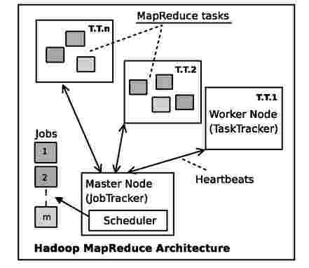
Fig. 1: Hadoop MapReduce Architecture
Hadoop borrows much of its architecture from the original MapReduce system at Google [12]. Figure 1 depicts the architecture of Hadoop's MapReduce implementation. Although the architecture is centralized, Hadoop is known to scale well from small (single node) to very large (upto 4000 nodes) installations [8]. HDFS (Hadoop Distributed File Systems) deals with storage and is based on the Google File System [14], and MapReduce deals with computation.
Each MapReduce job is subdivided into a number of tasks for better granularity in task assignment. Individual tasks of a job are independent of each other, and are executed in parallel. The number of Map tasks created for a job is usually proportional to size of input. For very large input size (of the order of petabytes), several hundred thousand tasks could be created [11].
Scheduling in Hadoop is centralized, and worker initiated. Scheduling decisions are taken by a master node, called the
JobTracker, whereas the worker nodes, called TaskTrackers are responsible for task execution. The JobTracker maintains a queue of currently running jobs, states of TaskTrackers in a cluster, and list of tasks allocated to each TaskTracker. Every TaskTracker periodically reports its state to the JobTracker via a heartbeat mechanism. The contents of the heartbeat message are:
• Progress report of tasks currently running on sender TaskTracker.
• Lists of completed or failed tasks.
• State of resources - virtual memory, disk space, etc.
• A boolean flag (acceptNewTasks) indicating whether the sender TaskTracker should be assigned additional tasks. This flag is set if the number of tasks running at the TaskTracker is less than the configured limit.
Task or worker failures are dealt by relaunching tasks. The JobTracker keeps track of the heartbeats received from the workers and uses it in task assignment. If a heartbeat is not received from a TaskTracker for a specified time interval, then that TaskTracker is assumed to be dead. The JobTracker then relaunches all the tasks previously assigned to the dead TaskTracker, that could not be completed. The Heartbeat mechanism also provides a communication channel between the JobTracker and a TaskTracker. Any task assignments are sent to the TaskTracker in the response of a heartbeat. The TaskTracker spawns each MapReduce task in a separate process, in order to isolate itself from faults due to user code in the tasks.
Data locality and speculative execution are two important features of Hadoop's scheduling. Data locality is about executing tasks as close to their input data as possible. Speculative execution tries to rebalance load on the worker nodes and tries to improve response time by relaunching slow tasks on different TaskTrackers with more resources.
The administrator specifies the maximum number of Map and Reduce tasks (mapred.map.tasks.maximum and mapred.reduce.tasks.maximum in Hadoop’s configuration files) that can simultaneously run on a TaskTracker. If the number of tasks currently running on a TaskTracker is less than this limit, and if there is enough disk space available, the TaskTracker can accept new tasks. This limit should be specified before starting a Hadoop cluster. This mechanism makes some assumptions which we find objectionable:
• In order to correctly set the limit, the administrator has detailed knowledge about the resource usage characteristics of MapReduce applications running on the cluster. Deciding the task limit is even more difficult in cloud computing environments such as the Amazon EC2, where the resources could be virtual.
• All MapReduce applications have similar resource requirements.
• The limit on max number of concurrent tasks correctly describes the capacity of a machine.
Clearly, these assumptions do not hold in real world scenarios given the range of applications for which Hadoop is becoming popular [7].As the above assumptions have been built into Hadoop, all the current schedulers available with Hadoop, the Hadoop default scheduler, FAIR scheduler [23], the capacity scheduler [3] and the dynamic priority scheduler [5] suffer from this limitation.
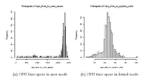
Fig. 2: CPU usage patterns of MapReduce applica-tion(wordcount). Mean and variance of the resource usage distributions become recognizable characteristics of a particular MapReduce job.
MapReduce applications have been successfully used in processing large amounts of data. Subtasks of the same type of a job apply the exact same computation on input data. Tasks tend to be I/O bound, with resource usages as a function of the size rather than the content of input data. As a result, the resource usage patterns of a MapReduce job tend to be fairly predictable. For example, in Figure 2, we show the CPU time spent in user mode and kernel mode by Map tasks of a WordCount job. The figure shows distribution of CPU usages for about 1700 Map tasks. As we can deduce from the figure, the resource usage of MapReduce applications follow recognizable patterns. Similar behavior is observed for other MapReduce apps and resource types. This, and the fact that the number of tasks increase with the size of input data, present a unique opportunity for using learning based approaches.
IV. Proposed algorithm
Having seen the scheduling mechanism in Hadoop, we explain our task assignment algorithm in this section. Our algorithm runs at the JobTracker. Whenever a heartbeat from a TaskTracker is received at the JobTracker, the scheduler chooses a task from the MapReduce job that is expected to provide maximum utility after successful completion of the task. Figure 3 depicts the task assignment process.
First, we build a list of candidate jobs. For each job in the queue of the scheduler, one candidate instance for Map part and one (or zero, if the job does not have a reduce part) for the Reduce part is added in the list. This is done because the resource requirements of Map and Reduce tasks are usually different.
We then classify the candidate jobs into two classes, good and bad, using a pattern classifier. Tasks of good jobs do not

Fig. 3: Task assignment using pattern classification. Evaluation of last decision, and classification for current decision are done asynchronously.
overload resources at the TaskTracker during their execution. Jobs labeled bad are not considered for task assignment. If the classifier labels all the jobs as bad, no task is assigned to the TaskTracker.
If after classification, there are multiple jobs belonging to the good class, then we choose the task of a job that maximizes the following quantity:
where, E.U.(J) is the expected utility, and U(J) is the value of utility function associated with the MapReduce job J. tj denotes a task of job J, and P (tj = good\Fl, F2,..., Fn) denotes the probability that the task tj is good. The probability is conditional upon the feature variables F1, F2,..., Fn. Feature variables are described in more detail later in this section.
Once a job is selected, we first try to schedule a task of the job whose input data are locally available on the TaskTracker. Otherwise, we chose a non data local task. This policy is the same as used by the default Hadoop scheduler.
We assume that the cluster is dedicated for MapReduce processing, and that the JobTracker is aware and responsible for every task execution in the cluster. Our scheduling algorithm is local as we consider state of only the concerned TaskTracker while making an assignment decision. The decision does not depend on state of resources of other TaskTrackers.
We track the task assignment decisions. Once a task is assigned, we observe the effect of the task from information contained in subsequent heartbeat from the same TaskTracker. If based on this information, the TaskTracker is overloaded, we conclude that last task assignment was incorrect. The pattern classifier is then updated (trained) to avoid such assignments in the future. If however, the TaskTracker is not overloaded, then
the task assignment decision is considered to be successful.
Users configure overload rules based on their requirements. For example, if most of the jobs submitted are known to be CPU intensive, then CPU utilization or load average could be used in deciding node overload. For jobs with heavy network activity, network usage can also be included in the overload rule. In a cloud computing environment, only those resources whose usage is billed could be considered in the overload rule. For example, where conserving bandwidth is important, an overload rule could declare a task allocation as incorrect if it results in more network usage than the limit set by the user.
The overload rules supervise the classifiers. But, as this process is automated, the learning in our algorithm is automatically supervised. The only requirement for an overload rule is that it can correctly identify given state of a node as being overloaded or underloaded. It is important that the overload rule remains the same during the execution of the system. Also, the rule should be consistent for the classifiers to converge.
During classification, the pattern classifier takes into account a number of features variables, which might affect the classification decision. The features we use are described below:
Job Features: These features describe the resource usage patterns of a job. These features could be calculated by analyzing past execution traces of the job. We assume that there exists a system which can provide this information. In absence of such a system, the users can utilize these features to submit 'hints' about job performance to the classifier. Once enough data about job performance is available, user hints could be mapped to resource usage information. The job features we consider are: job mean CPU usage, job mean network usage, mean disk I/O rate, and mean memory usage. The users estimate the usages on the scale of 10. A value of 1 for a resource means minimum usage, whereas 10 corresponds to maximum usage. For a given MapReduce job, the resource usage variables of the Map part and the Reduce part are considered different.
Node Features (NF): Node features denote the state and quality of computational resources of a node. Node Static Features change very rarely, or remain constant throughout the execution of the system. These include number of processors, processor speed, total physical memory, total swap memory, number of disks, name and version of the Operating System at the TaskTracker, etc. Node Dynamic Features include properties that vary frequently with time. Examples of such properties are CPU load averages, % CPU usage, I/O read/write rate, Network transmit/receive rates, number of processes running at the TaskTracker, amount of free memory, amount of free swap memory, disk space left etc. Processor speed could be be a dynamic feature on nodes where CPUs support dynamic frequency and voltage scaling.
Utility functions are used for prioritizing jobs and policy enforcement. An important role of the utility functions is to
make sure that the scheduler does not always pick up ‘easy’ tasks. If the utility of all the jobs is same, the scheduler will always pick up tasks that are more likely to be labeled good, which are usually the tasks that demand lesser resources. Thus, by appropriately adjusting job utility it could be made sure that every job gets a chance to be selected.
It is possible that a certain job is always classified as bad regardless of the values of feature vectors. This could happen if the resource requirements of the job are exceptionally high. However, this also indicates that the available resources are clearly inadequate to complete such a job without overloading.
Utility functions could also be used in enforcing different scheduling policies. Examples of some such policies are given below. One or more utility functions could be combined in order to enforce hybrid scheduling policies.
1) Map before Reduce: In MapReduce, it is necessary that all Map tasks of a job are finished before Reduce operation begins. This can be implemented by keeping the utility of Reduce tasks zero until a sufficient number of Map tasks have completed.
2) First Come, First Serve (FCFS or FIFO): FCFS policy can be implemented by keeping the utility of the job proportional to the age of the job. Age of a job is zero at submission time.
3) Budget Constrained: In this policy, tasks of a job are allocated until the user of a job has sufficient balance in his/her account. As soon as the balance reaches zero, the utility of jobs of the said user becomes zero, thus no further tasks of jobs from the said user will be assigned to worker nodes.
4) Dedicated Capacity: In this policy a job is allowed a guaranteed access to a fraction of the total resources in the cluster. Here, the utility could be inversely proportional to the deficit in the currently allocated fraction, and the promised fraction. Utility of jobs allocated more than the promised fraction is set to zero to make sure that they are not considered during task assignment.
5) Revenue oriented utility: In this policy, utility of a job is directly proportional to the amount the job’s submitter is willing to pay for successful completion of the job. This makes sure that the algorithm always picks tasks of users who are offering more money for the service.
Next, we explain how the same algorithm can be implemented by using two different pattern classifiers. In this paper we consider only the Naive Bayes Classifier, and the Perceptron classifier [13]. Theoretically, any linear classifier could be used for classifying jobs. However, we discuss these two based on their ease of implementation, and the ability of learning from one sample at a time (online learning). Online learning helps in keeping memory used by the classifiers constant w.r.t the number of feature vectors. This is essential in our case; efficiency is an important goal for a scheduler implementation.
C. Using a Naive Bayes Classifier If we apply Bayes theorem to equation 1 mentioned in the beginning of this section, we get,

The denominator in the above equation can be treated as a constant as its value is independent of the jobs, and thus its calculation can be skipped during comparison.
We calculate both P(tj = good|Fi, F2,...,Fn) and P(tj = bad|Fi, F2,..., Fn). Job is labeled as good or bad depending on which of the two probabilities is higher. Under the assumption of Naive Bayes conditional independence we get,

Thus, we compute the following quantity for all the jobs and select the job that maximizes it.

Once the effects of a task assignments are observed, the probabilities are updated accordingly so that future decisions could benefit from the lessons learnt from the effects of current decisions.
Here we assume that the probabilities of all feature variables are conditionally independent of each other. This may not always be true. However, we observed that this assumption can yield a much simpler implementation. Despite the assumption, Naive Bayes classifiers are known to perform well. Our results show that the assumption does not have any drastic undesired effects on the overall performance of the scheduler.
D. Using a Perceptron Classifier
Using a perceptron classifier, a job in the scheduler’s queue is considered good if the result of the classification function c, is one and bad if the output is zero. Input to the classification function is the feature vector F.

Here, F is the feature vector comprising of feature variables described earlier in this section. W is the vector of weights assigned to each connection in the perceptron. b is a constant term that does not depend on any feature vector. W.F gives the dot product of the two vectors. If the product is greater than -b, the job is labeled as good, otherwise it is labeled as bad. Figure 4 shows a perceptron classifier.
Initially all the weight variables are set to zero. Based on the result of applying the overload rule (after the next heartbeat from the TaskTracker is received), the weights are updated as follows:
for j = 1.. . n; n being the number of feature variables. Wj and Fj are the corresponding elements of the weight vector and feature vector respectively. y gives the result after applying the overload rule to the state of TaskTracker, which is 1 if the TaskTracker is underloaded, and 0 if it is overloaded. The weights are updated only if the predicted class label (c(F)) is different from the desired class label (y). a is the learning rate, which is set to one.
E. Separability of feature vector space and classifier convergence
Naive Bayes classifiers assume that all feature variables are conditionally independent of each other, and their probabilities could be calculated independently. This assumption is almost always incorrect in practice. However, Naive Bayes classifiers have been known to outperform other popular classifiers including decision trees and multilayer neural networks. Zhang [24] has discussed in detail about the unexpected efficiency of Naive Bayes classifiers.
Convergence of a linear classifier such as a perceptron depends on the separability of feature vector space. For linearly separable classes, perceptron classifier is known to learn the class boundary within a finite number of iterations [13]. Here, we argue about the separability of vector space of the feature variables that we consider while making a classifier decision.
All the feature variables used in our classifier indicate either availability or usage of computational resources at a given node. Clearly, more the availability of a resource, more is the likelihood of a task being completed without overloading the resource. For features which correspond to usage of resources, such as the job features, the opposite is true. i.e., more the resource usage, more is the likelihood of task of that job overloading the node. Thus, we can say that for a given job, for every feature variable there exists a separating value on one side of which task of the job is likely to overload the node, and vice versa. The vector corresponding to all such separating values gives the hyperplane which separates the feature vectors into two classes, good, and bad.
V. EVALUATION AND RESULTS
We now briefly discuss the implementation, and then explain the evaluation methodology and results of our experiments in this section.
A. Implementation Details
We have implemented our algorithm for Hadoop version 0.20.0. Our scheduler uses the pluggable scheduling API introduced in Hadoop 0.19. The scheduler customizes assignTasks method of the
org.apahce.hadoop.mapred.TaskScheduler
class.
We used only the Naive Bayes classifier in our implementation. Naive Bayes classifier is better in online learning (learning from one sample at a time) and handling categorical feature variables compared to perceptron classifier. We used a simple histogram for counting probabilities of discrete features.
Node Features are obtained from the heartbeat message. We extended the heartbeat protocol used in Hadoop to include node resources properties. Job Features are passed via a configuration parameter (leansched.jobstat.map and learnsched.jobstat.reduce) while launching a job. In absence of these parameters, mode of the values for each resource is considered as the respective job feature.
At any point of time, we maintain at the most k decisions made by the classifier for each TaskTracker, where k is the number of tasks assigned in one heartbeat. During the evaluation we kept k = 1. Once the decisions are evaluated by the overload rule, we persist them to disk so that they can be used in re-learning, or when the desired utilization level is changed by the user. A decision made for the current heartbeat is evaluated in the next heartbeat. This allows us to control the memory used by decisions. We disregard the accpetNewTasks flag in the heartbeat message, and consider a node for task assignment in every heartbeat.
We allow users to implement their own utility functions by extending our API. Utility functions in the scheduler are pluggable and can be changed at runtime. We have implemented a constant utility function, and FIFO utility function. Users can also write their own overload rules by implementing the DecisionEvaluator interface.
B. Evaluation Methodology and Workload description
We used a cluster of eight nodes to evaluate our algorithm. One of the nodes was designated as the master node which ran HDFS and MapReduce masters (NameNode and JobTracker). The remaining seven nodes were worker nodes. All of the nodes had 4 CPUs (Intel Quad Core, 2.4 GHz), a single hard disk of capacity 250 GB, and 4 GB of RAM. The nodes were interconnected by an unmanaged gibabit Ethernet switch. All of the nodes had Ubuntu Linux (9.04, server edition) and SUN Java 1.6.0_13. We used Hadoop version 0.20.0 for this evaluation. The important Hadoop parameters and their values used in the experiments are described in Figure 5. For rest of the parameters, we used Hadoop’s default values.
We used one minute CPU load averages to decide overloading of resources. Load averages summarize both CPU and IO activity on a node. We calculated the ratio of reported load average with the number of available processors in a node. A value of 1 for this ratio indicates 100% utilization on a node.
A node was considered to be overloaded if the ratio crossed a user specified limit.
We evaluated our scheduler using jobs that simulate real life workloads. In addition to the WordCount and Grep jobs used by Zaharia et. al. [22], we also simulate jobs to represent typical usage scenarios of Hadoop. We collected Hadoop usage information from the Hadoop PoweredBy [7] page. This page lists case studies of over 75 organizations. We categorized the usages into seven main categories, text indexing, log processing, web crawling, data mining, machine learning, reporting, data storage and image processing. Figure 6 summarizes the frequency of these use cases. The percentages represented in the figure are approximate. From this information, we conclude that Hadoop is being used in a wide range of scenarios, naturally creating diversity in the resource requirements of MapReduce jobs.

Fig. 6: Prominent Use Cases for Hadoop. (percentages are approximate)
We came up with the following set of jobs to evaluate our scheduler. We describe their functioning below:
• TextWriter: Writes randomly generated text to HDFS. Text is generated from a large collection of English words.
• WordCount: Counts word frequencies from textual data.
• WordCount with 10 ms delay: Exactly same as Word-Count, except that we add an additional sleep of 10 ms before processing every key-value pair.
• URLGet: This job mimics behavior of the web page fetching component of a web crawler. It downloads a text file from a local server. The local server delays response for a random amount (normal distribution, ^ = 1.5s, a = 0.5s) of time to simulate internet latency. The text files we generated had sizes according to normal distribution
|
Job |
CPU |
Memory |
Disk |
Network |
|
TextWriter |
3 |
5 |
5 |
3 |
|
WordCount |
5 |
6 |
8 |
5 |
|
WordCount+10ms delay |
1 |
6 |
6 |
4 |
|
URLGet |
3 |
4 |
6 |
7 |
|
URLToDisk |
3 |
5 |
7 |
8 |
|
10 |
5 |
5 |
3 |
Fig. 7: Resource usage of evaluation jobs as estimated on the scale of 10, a value of 1 indicates minimum usage
with mean of 300 KB, and variance of 50 KB [17]. URLToDisk: Downloads large video files(200MB) from a local web server and saves them to disk.
CPUActivity: Carries out a computationally expensive numerical calculation for every key-value pair in the input.
|
Hadoop Parameter |
Value |
|
Replication |
3 |
|
HDFS Block size |
64 MB |
|
Speculative Execution |
Enabled |
|
Heartbeat interval |
5 seconds |
We estimated the resource usages of the each job profile thus created on a scale of 10 based on empirical observations for each computational resource. These values are shown in Figure 7. A value of 10 for a resource means maximum resource usage. These estimates were passed to the scheduler as Job Features as discussed in Section IV-A. It should be noted that the approximate usage estimates could be replaced by actual estimates if such information is available. Our algorithm will work in both cases, provided the estimates are mapped properly to actual resource usages.
During each run of a job the input was created afresh, and deleted after the job was completed using the RandomTextWriter job in Hadoop. The job generated 10 GB of text from words randomly chosen from a large collection of English words.
C. Results
We first demonstrate the learning behavior of the scheduler. In this experiment we ran the WordCount MapReduce job provided in Hadoop. The job was run several times on randomly generated text of size 70 GB. The input was regenerated before each run of the job. Figure 8a shows the average load on one of the worker nodes during this period.
The scheduler was asked to maintain utilization at 100%. Initially the utilization was lower than expected during the ‘learning phase’ of the scheduler. After that however, the nodes were rarely overloaded, and achieved utilization very close(approx. 96%) to the desired value(100%). Another interesting observation is that the intensity of ‘peaks’ in the load reduces with time, thus confirming that the scheduler is indeed learning.
Figure 8b shows the reduction in the runtime of WordCount during this period. We report only the first six runs, since after that the runtime converged to around 36 minutes. The scheduler converges in the first few runs of the job, with the greatest reduction between the first two runs. The large runtime of the first run is due to the underutilization during the learning phase of the scheduler. We would like to point out that for larger jobs, i.e. for jobs with more number of Map tasks, the scheduler would converge even quickly.

Fig. 8: Learning behavior of the scheduler for WordCount job
Next, we evaluated whether the scheduler is able to achieve user specified utilization. For this experiment we used Tex-tWriter, WordCount and Grep jobs. A constant utility function was used to make sure that all the jobs had equal priority. During each run, we first ran the TextWriter job to create input before running WordCount and Grep. We changed the desired utilization ratio (ratio of 1 means maintaining 100% utilization, which in turn means maintaining load average of 4 on a quad core machine) from 1 to 4 in steps of 0.5.
Figure 9 shows the observed behavior of the scheduler. The figure shows mean load averages and variations in a single run. The values reported are averaged over ten experiments. As is shown in the figure, the achieved load average is quite close to the desired load average (4 times x). The relatively large variation in the values can be attributed to the initial underutilization during the learning phase of the scheduler. For higher values of desired utilization ratio, the gap between desired and achieved load averages increases. This is because it is difficult to maintain work at higher utilization, as we can assign a task only every 5 seconds (heartbeat interval).
We have deliberately included the learning phase of the scheduler in our evaluations, for comparing the scheduler fairly

Fig. 9: Achieved utilization for different user requirements
with Hadoop's default scheduler, as the default scheduler does not involve any learning phase.

Fig. 10: Classifier accuracy for URLGet and CPUActivity
Next, we compare the learning rates of two jobs, URLGet and CPUActivity. URLGet is a network intensive job, whereas CPUActivity is CPU intensive. We report accuracy of the decisions made by the classifier in Figure 10. We consider a decision to be accurate if it is validated by the overload rule. For example, a decision to allocate a task is accurate if the overload rule determines that the allocation did not cause any overload. We report percentage accuracy per 250 decisions made by the classifier. The accuracy for both the jobs increases, which is expected as the scheduler is learning about the impact of both jobs on utilization. However, the rate of increase in URLGet is much smaller compared to CPUActivity. This could be because of the delayed response by local servers in case of URLGet. As the request from local server is delayed, URLGet tends to block for network I/O for rather unpredictable duration. CPUActivity on the other hand tends to be more predictable, and hence classifier accuracy for CPUActivity improves faster. Another point to note is that achieving 100% accuracy is not that important as long as the scheduler is able to maintain utilization level specified by the user. Also, achieving 100% accuracy could be difficult, because of uncertainty involved in factors such as utilization contributed by DataNode processes, network traffic, age of resource information [18], and finally errors in estimating resource requirements of jobs.
We now present the last set of our experiments in which we compared our scheduler against Hadoop’s native scheduler described in Section III. For these experiments, we used the workload as described in Section V. Again, we used a constant utility function. We did not use any policy scheme (as described in Section IV-B), as our goal was to demonstrate that our scheduler does better task assignment than Hadoop’s native scheduler. We do not compare our scheduler with other Hadoop schedulers because the number of tasks assigned by them would be the same as that by the default scheduler because of reasons discussed in Section III. Each of the jobs was run in isolation. Input was regenerated before every new run of a job.
We set the maximum number of concurrent tasks to 5 (4CPUs + 1 disk). This was done to make sure that each task always had access to a disk or a CPU. This setting does not apply to the learning scheduler. Note that this is larger than the default Hadoop setting, where only two tasks are allowed to run concurrently on a machine.
|
Job |
Learning Scheduler |
Hadoop native |
Runtime compared to Hadoop |
|
TextWriter |
2.03 |
5 |
2.5x |
|
WordCount |
2.31 |
5 |
2x |
|
WordCount + 10ms delay |
10.52 |
5 |
0.4x |
|
URLGet |
8.35 |
5 |
0.6x |
|
URLToDisk |
5.09 |
5 |
1x |
|
3.17 |
5 |
1.5x |
Fig. 11: Comparison of task assignment by Learning Scheduler and Hadoop’s native scheduler
Figure 11 shows the mean number of tasks assigned during each run by our scheduler and Hadoop’s default scheduler. The values are averages calculated over 10 experiment runs. Our scheduler allocated tasks in order to maintain utilization of 100%. Job runtime is proportional to the number of tasks assigned by learning scheduler and Hadoop default, as we made sure that each of the task would take 60 seconds to complete. As can be seen from the table, Hadoop’s scheduler achieved better runtime in TextWriter, WordCount and CPUAcitivity jobs. However, it should be noted that in all these cases, Hadoop’s task assignment policy resulted in overload at the worker machines due to excessive task assignment. Since our scheduler assigns tasks by considering utilization, shorter runtime could be easily achieved if the utilization target given to the scheduler is increased. For WordCount with 10 ms delay, URLGet and URLToDisk the learning scheduler achieved significantly shorter runtime than the comparison. This is because, Hadoop allocated only fixed number of tasks, whereas our scheduler could allocate more tasks as each task was less demanding. The biggest improvement is seen in
WordCount with 10 ms delay. For these jobs, in the case of default Hadoop scheduler, the cluster was underutilized.
In the next section we conclude our discussion by mentioning key lessons learnt and directions of further research.
VI. Conclusions and Future work
We presented a new algorithm for task assignment using machine learning. Our work shows that learning based techniques can be effectively used in tackling distributed resource management. A key property of our scheduler was continuous learning and adaptation for heterogeneous workloads. Despite the uncertainty involved in clusters, the scheduler was able to learn impact of different applications in their first few runs. We would like to point out that the jobs we used for evaluation were of rather modest sizes when compared to the real life MapReduce case studies. However, this is in fact beneficial to our algorithm as with large applications we have even better opportunity to build models on job performance data. For large applications the scheduler could learn the behavior in the first run itself.
Once the scheduler stabilizes, we achieved much better performance than the default Hadoop scheduler. However, as the underutilization in the learning phase is a limitation specific to our algorithm and not the default scheduler, we have included it in our results.
The key lessons learnt from our work are, that even simple learning based approaches such as the Naive Bayes classifier could be used in optimizing repetitive workloads. Another important lesson is that prediction based task assignment results in better utilization of cluster hardware.
The algorithm we have presented is generic and can be applied to other resource management problems as well. For example the same approach could be used in solving admission control, where a controller has to selectively choose among incoming jobs. Speculative execution is also a problem where we would like to use this approach.
In the future we would like to evaluate our scheduler in heterogeneous environments as well as in cloud computing environments such as the Amazon EC2. Incorporating features that indicate node stability, and predicting component failures is another interesting future direction.
References
[1] Amazon Elastic MapReduce. http://aws.amazon.com/elasticmapreduce/.
[2] Apache Hadoop. http://hadoop.apache.org.
[3] Capacity Scheduler for Hadoop. http://hadoop.apache.org/common/docs/ current/capacity_scheduler.html.
[4] Cloudera Distribution for Hadoop on EC2. http://www.cloudera.com/ hadoop-ec2.
[5] Dynamic Priority Scheduler for Hadoop. http://issues.apache.org/jira/ browse/HADOOP-4768.
[6] Hadoop on Demand. http://hadoop.apache.org/common/docs/current/ hod_user_guide.html.
[7] Hadoop PoweredBy. http://wiki.apache.org/hadoop/PoweredBy.
[8] Scaling Hadoop to 4000 nodes at Yahoo! http://developer.yahoo.net/ blogs/hadoop/2008/09/scaling_hadoop_to_4000_nodes_a.html.
[9] Amy W. Apon, Thomas D. Wagner, and Lawrence W. Dowdy. A learning approach to processor allocation in parallel systems. In CIKM '99: Proceedings of the eighth international conference on Information and knowledge management, pages 531-537, New York, NY, USA, 1999. ACM.
[10] Z. Bin, L. Zhaohui, and W. Jun. Grid Scheduling Optimization Under Conditions of Uncertainty. Lecture Notes in Computer Science, 4672:51, 2007.
[11] J. Dean. Experiences with MapReduce, an abstraction for large-scale computation. In International Conference on Parallel Architecture and Compilation Techniques, 2006.
[12] Jeffrey Dean and Sanjay Ghemawat. MapReduce: Simplified Data Processing on Large Clusters. In Proceedings of the 6th Symposium on Operating Systems Design and Implementation, pages 137-150, 2004.
[13] Richard O. Duda, Peter E. Hart, and David G. Stork. Pattern Classification (2nd Edition). Wiley-Interscience, 2 edition, November 2000.
[14] Sanjay Ghemawat, Howard Gobioff, and Shun-Tak Leung. The google file system. SIGOPS Oper. Syst. Rev., 37(5):29-43, 2003.
[15] T. Kunz. The Learning Behaviour of a Scheduler using a Stochastic Learning Automation. Technical report, Citeseer.
[16] T. Kunz. The influence of different workload descriptions on a heuristic load balancing scheme. IEEE Transactions on Software Engineering, 17(7):725-730, 1991.
[17] Ryan Levering and Michal Cutler. The portrait of a common HTML web page. In DocEng ’06: Proceedings of the 2006 ACM symposium on Document engineering, pages 198-204, New York, NY, USA, 2006. ACM.
[18] Michael Mitzenmacher. How useful is old information? IEEE Trans. Parallel Distrib. Syst., 11(1):6-20, 2000.
[19] A. Negi and K.P. Kishore. Applying machine learning techniques to improve linux process scheduling. In TENCON 2005 2005 IEEE Region 10, pages 1-6, Nov. 2005.
[20] L.P. Santos, D. de Informatica, and A. Proenca. A Bayesian runtime load manager on a shared cluster. In First IEEE/ACM International Symposium on Cluster Computing and the Grid, 2001. Proceedings, pages 674-679, 2001.
[21] L.P. Santos and A. Proenca. Scheduling under conditions of uncertainty: a bayesian approach. Lecture notes in computer science, pages 222-229, 2004.
[22] M. Zaharia, A. Konwinski, A.D. Joseph, R. Katz, and I. Stoica. Improving mapreduce performance in heterogeneous environments. In Proc. of USENIX OSDI, 2008.
[23] Matei Zaharia, Dhruba Borthakur, Joydeep Sen Sarma, Khaled Elmele-egy, Scott Shenker, and Ion Stoica. Job Scheduling for Multi-User MapReduce Clusters. Technical Report UCB/EECS-2009-55, EECS Department, University of California, Berkeley, Apr 2009.
[24] Harry Zhang. The Optimality of Naive Bayes. In Valerie Barr and Zdravko Markov, editors, FLAIRS Conference. AAAI Press, 2004.