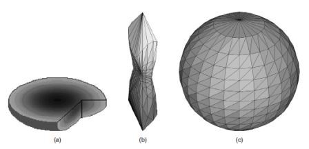
Figure 1. Overcoming the problem of anisotropic sampling: (a) An image with isotropic sampling, subsequently subsampled with rates 1:2:3. (b) Orientation if the anisotropic sampling is ignored. (c) Its orientation indicatrix if scaling is used
Abstract: Will be presented some of the recent developments in the field of computational models for brain image analysis. Computational neuroanatomical models will evolve in various directions during the next decade. The main foundation that allows investigators to examine brain structure and function in precise, quantitative ways has already been laid.
Key words: brain tissue, image analyze, neuroanatomical models, 3D representation, texture analize.
Introduction. In recent years there is a proliferation of sensors that create 3D images
, particularly so in medicine.
These sensors either operate in the plane, creating slices of data which, if dense enough, can be treated as volume data, or
operate in the 3D space directly, like some new PET sensors which reconstruct volume data by considering out of plane coincident events.
Either way, one may end up having measurements that refer to positions in the 3D space. Hitherto such data have been analysed and viewed as 2D
slices. This is not surprising: apart from the fact that often only sparse slices were available, even when volume data existed, the analysis and
visualisation has been inspired by the limited abilities of human perception: the human eye cannot see volume data, yet alone analyze them. However,
this way a large part of the information content of the data is totally ignored and unutilised. Computerised analysis offers the exciting option of
escaping from the anthropocentric description of images, and go beyond the limitations of the human visual and cognitive system. I present some
techniques appropriate for the texture analysis of volume data in the context of medical applications. The microstructural features that can be
calculated this way offer a totally new perspective to the clinician, and the exciting possibility of identifying new descriptions and new indicators
which may prove valuable in the diagnosis and prognosis of various conditions. In particular, I shall express the variation of the data along different
orientations using two versions of the so called orientation
histogram. First, we shall discuss ways by which one can construct and visualise the
orientation histogram of volume data. Then I shall concentrate on the calculation of features from the orientation histogram, and in particular features
that encapsulate the anisotropy of the texture. Finally we shall present some examples of applying these techniques to medical data.
Issues Related to 3D Texture Estimation and Representation. There are three major issues related to the calculation and visualisation of a 3D orientation histogram:
The first two topics have been extensively discussed in relation to 3D object representation (e.g., [1]), while the third is intrinsic to the medical topographic data acquisition protocols.
The problem of anisotropic sampling is relevant when metric 3D calculations are performed with the image. As the creation of features from the orientation histogram necessarily involves metric calculations, the issue of anisotropic sampling is important. It is a common practice when acquiring tomographic data to choose slice separation much larger than the pixel size on each slice. Thus, the voxels of the acquired image in reality are not cubes but elongated rectangular parallelepipeds with the longest side along the z axis, i.e., the axis of slice separation. The metric used for the various calculations then is the Euclidean metric with a scaling factor multiplying the z value to balance this difference.
3D Texture Representation. The first texture descriptor we shall examine is based on a gradient density
(GD) measure, while the second on an intensity variation
(INV) measure.
Figure 1. Overcoming the problem of anisotropic sampling: (a) An image with isotropic sampling, subsequently subsampled with rates 1:2:3. (b) Orientation if the anisotropic sampling is ignored. (c) Its orientation indicatrix if scaling is used
Gradient Density Measures (GD). The 2D optimal
filters that have been developed for 2D edge detection (e.g., [2]) are not appropriate for estimating
the local gradient in textured images due to the multiplicity of edges present in them. Much more appropriate are small filters that avoid the problem of
interference. Such a filter for 3D images has been proposed by Zucker and Hummel [3].
This filter is 3☓3☓3 in size, and is represented here by its three cross‑sections orthogonal to the direction of convolution:
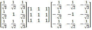
Figure 2. Zucker and Hummel filter
The convolution of the image with this mask along the three axes produces the three components of the gradient vector at each voxel. Two versions of the orientation histogram are then possible. Each gradient vector calculated is assigned to the appropriate bin of the histogram, and the bin value is incremented by the magnitude of the gradient vector. Alternatively, the bin of the orientation histogram may be accumulated by 1 every time a vector is assigned to it, irrespective of the magnitude of that vector. The latter approach was proved more robust when the weakest 5‑7% of the gradient values were trimmed off when the orientation histogram was created, due to the fact that such gradient vectors have very poorly defined orientations.
Intensity Variation Measure (INV). This method is based on the 3D version of the Spatial Gray‑Level Dependence Histogram (SGLDH). For this purpose, Chetverikov’s 2D approach [4] is generalised to 3D for arbitrary relative positions of the compared density values.
First we define the five‑dimensional co‑occurrence histogram with elements that count the number of pairs of voxels that appear at a certain relative position with respect to each other and have certain grey values. For example, element h(i, j, f, z, d) of this histogram indicates the number of pairs of voxels that were found to be distance d apart, in the (f, z) direction, and have density values i and j respectively. The value of the image at non‑integer positions is obtained by trilinear interpolation: The grey value at a general position (x, y, z) is assumed to be a trilinear function of the position itself, i.e.,

Figure 3. Trilinear function of the position.
where a1 , ... , a8 are some parameters. The values of these parameters are determined from the known values at the eight integer positions that surround the general position
Figure 4. Integer positions that surround the general position
Following Conners and Harlow [5], we define the inertia of the image with the help of this histogram, as follows:

Figure 5. Inertia of the image
where Ng is the number of grey values in the image, and we have used a semi‑colon to separate d from the rest of the variables in order to indicate that in our calculations we shall keep d fixed. We use I(φ, z; d) to characterize the texture of the image and visualize it as a 3D structure showing the magnitude of I(φ, z; d) in the direction (φ, z).
In practice, of course, we never construct the 5‑dimensional array h(i, j, φ, z; d). Instead, we fix the value of d and the values of the directions (φ, z) at which function I(φ, z; d) will be sampled. Then, each voxel is visited in turn and its pair location is found at the given distance and given direction; the grey value at that location is calculated, its difference from the grey value of the voxel is found, it is squared and accumulated. This is repeated for all chosen sampling directions (φ, z). These directions could, for example, be the centers of the bins used for the GD method. However, there is a fundamental difference in the nature of the two approaches: In the GD approach, the more directions we choose, the larger the number of bins we have to populate by the same, fixed number of gradient vectors. As a result, the more bins we have, the more rough and noisy the indicatrix looks because the number of vectors we have to populate them with becomes less and less sufficient. The more sampling points we choose, the better the function is sampled and the smoother it looks.
Quantifying Anatomy via Shape Transformations. This section presents a general mathematical framework for representing the shape characteristics of an individual’s brain. Since this framework is based on a shape transformation, we first define exactly what we mean by this term. Consider a three‑dimensional (volumetric) image, I, of an individual’s brain. Let each point in this image be denoted by x=(x, y, z)T. A shape transformation, T, of I is a map that takes each point x∈I and maps it to some point T(x). In the context of development, x belongs to the brain of one individual, and T(x) belongs to the brain of another individual. Moreover, these two points are homologous to each other. In other words, the transformation T is not just any transformation that morphs one brain to another, but it is one that does this morphing so that anatomical features of one brain are mapped to their counterparts in another brain.

Figure 6. (a,b) A network of curves (sulci) overlaid on 3D renderings of the outer brain boundaries of two individuals
Several investigators have used shape transformations to study brain anatomy [6–10]. However, this approach has its roots in the early century’s seminal work by D’Arcy Thompson [11], who visualized the differences between various species by looking at transformations of Cartesian grids, which were attached to images of samples from the species. Although D’Arcy Thompson, with his insightful analysis, placed the roots for modern computational anatomy, his vision came short of realizing that this technique can be far more powerful than merely quantifying gross morphological differences across species. The reason is that modern image analysis techniques have made it possible to morph one anatomy to another with much higher accuracy than D’Arcy Thompson’s transformations.
In order to provide the understanding of how one can precisely quantify the anatomy of an individual brain, let’s draw upon an analogy from a standard measurement problem: How do we measure the length of an object? Three steps are involved. First, we need to define a standard, a measurement unit. What exactly we choose as our unit is relatively unimportant; it can be the meter, the inch, or any other unit of length. However, we do need to have a unit, in order to be able to place a measurement in a reference system. Second, we need to define a way of comparing the length of an object with the unit; we do this by stretching a measure over the object, and measuring how many times our measure fits into the object’s length. Third, we need to define a means of comparing the lengths of two objects; this is what the arithmetic of real numbers does. For example, a 3‑meter object is longer than a 2‑meter object. Note that we cannot directly compare 3 meters with 15 inches; we first need to place both measurements in the same measurement system. A generalization of the comparison between two lengths, which is of relevance to our discussion, is the comparison of two groups of lengths. For example, we might want to know if nutrition and other factors have an effect on a population’s height. Standard statistical methods, such as t‑tests or an analysis of variance, will do this, by taking into consideration the normal variability of height within each population.
Placing this analogy in the context of computational neuroanatomy, we need three steps in order to construct a representation of an individual’s anatomy.
First, we must choose a unit. Here, the unit is a template of anatomy, perhaps an anatomical atlas [12] or the result of some statistical averaging procedure
yielding an average brain
[8]. Second, we need to define a procedure for comparing an individual brain with the template. This is accomplished via a
shape transformation that adapts the template to the shape of the brain under analysis. This shape transformation is analogous to the stretching of a
measure over the length of an object. Embedded in this transformation are all the morphological characteristics of the individual brain, expressed with
respect to those of the template. Finally, the third component necessary for shape comparisons is a means of comparing two brains whose morphology has
been represented in terms of the same unit, i.e., in terms of the same template. This can be accomplished by comparing the corresponding shape
transformations. The goal here is to be able to put in numbers the shape differences between two synthesized objects, using this particular template as
the measurement unit. In particular, the
color code re?ects the amount of stretching that the template had to undergo in order to be adapted to each of the two shapes.
Conclusion. We demonstrated some different approaches to analysing 3D textures. For most of our experiments with real data the gradient method was adopted, as it was also more appropriate for the analysis of the micro‑textures that are present in medical images. The robustness of the INV method on the other hand, makes it more appropriate for the global description of macro‑textures. The methodology presented here is generic and it has already been used in some medical studies.
Modern computational models for brain image analysis have made it possible to examine brain structure and function in greater detail than was possible via traditionally used methods. For example, such models will soon allow us to obtain structural and functional measurements regarding individual cortical gyri or sulci, not merely of larger structures such as lobar partitions of the brain. Moreover, we will be able to perform such measurements on large numbers of images because of the high degree of automation of algorithms emerging in this field.
Such works demonstrate the potential of such an analysis in 1) diagnosing a pathology 2) quantifying the severity of the pathology 3) quantifying the change with time of a certain pathological condition, or structural tissue characteristics.