Energy Capacity Reduction of Energy Storage System in Microgrid by Use of Heat Pump. Characteristic Study by Use of Actual Machine.

Автор: S. Kawachi, J. Baba, H. Hagaiwara, E Shimoda, S. Numata, E Masada, T Nitta
Источник: 14th International Power Electronics and Motion Control Conference, EPE-PEMC 2010

Abstract

S. Kawachi, J. Baba, H. Hagaiwara, E Shimoda, S. Numata, E Masada, T Nitta Energy Capacity Reduction of Energy Storage System in Microgrid by Use of Heat Pump –Characteristic Study by Use of Actual Machine. The installation of renewable energy sources based generators such as photovoltaic cells and wind turbines require energy storage systems (ESSs) to control power fluctuation. ESSs, however, are quite expensive. In order to reduce the necessary capacity of ESSs for microgrid applications, the control of heat pumps is researched. In this research, basic characteristic of a heat pump's power consumption is measured experimentally by use of heat pump chiller unit used in real building. Using the measured characteristic, a method to reduce the energy capacity of ESS is proposed and studied. The capacity reduction of ESS that can be achieved by use of heat pump control and the effect of control on temperature were calculated using simulations.

I. Introduction.

A. Background.

Today, the global climate change is an issue of high importance that demands the reduction of greenhouse gas emission urgently. Meantime power conversion by use of semiconductor devices is becoming more and more attractive by development of power electronics technology. In such background, generation from renewable energy sources through photovoltaic cells(PVs) and wind turbines(WTs) in the power grid is increasing. However, the generation from these renewable energy sources are random and intermittent in nature. When these fluctuations become substantial, it will be difficult to maintain the balance between power supply and demand.

The compensation of power fluctuation using energy storage systems(ESSs) is an effective solution to this problem. In previous research, authors proposed a control method of distributed generation systems(DGs) to compensate power fluctuations in a microgrid and verified its effectiveness experimentally using real machines[1],[4].

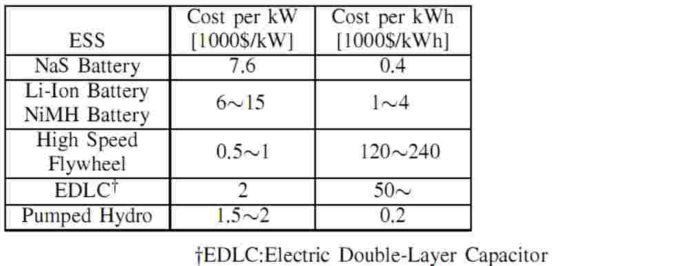
It is, however, preferable to keep installed capacity of ESSs as small as possible, since ESSs are generally expensive. Table I shows example of several ESSs' costs per output power(kW) and costs per energy(kWh)[5]. Figures show that most ESSs' costs are still quite high.

Many studies have been done to develop ways to reduce the capacity of ESSs. In case of wind turbine, control of blade pitch angle can reduce the power fluctuation and thus reduce the ESSs' capacity[6]. Also, accurate forecasting of renewable energy source's output power has possibilities to reduce ESSs.

Table I – Example of ESS's cost.

B. Concept of Controllable Load.

As another way of reducing the capacity of ESSs that is necessary for compensation of power fluctuation, controlling electrical appliances on the demand side is considered. In this paper, electrical appliances that can be controlled are called controllable load

.

There are several requirements for an electrical appliance to be treated as controllable load. They are:

1) The power consumption of the appliance should be large enough so that control of power consumption can compensate power fluctuation.

2) The response speed of the appliance’s power consumption to its reference signal should be fast enough to compensate power fluctuation.

3) Control of power consumption should not give inconvenience to the user of the appliance.

C. Heat Pump as Controllable Load.

Among electrical appliances, heat pumps, which are used for air conditioning and water heating and so on, are attractive options for control and is likely to satisfy the three requirements mentioned in previous section [2].

To evaluate heat pump’s conformity to requirement 1), number and types of air conditioning equipments used in Japan were surveyed. Figs. 1 and 2 show breakdowns of air conditioning equipments in residential and commercial sector respectively. Graphs indicate that there is a large percentage of heat pumps used for air conditioning. Thus, a large scale regulating capacity for power fluctuation

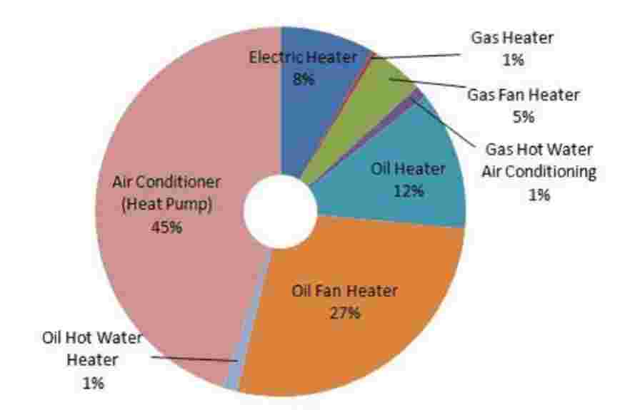
Figure 1 – Percentage of air conditioning equipments in residential sector in Japan in 2006.

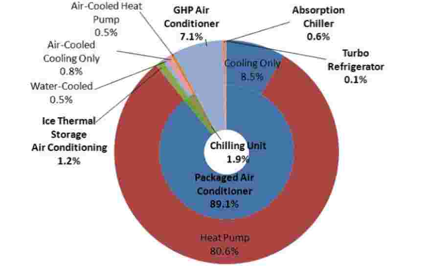
Figure 2 – Percentage of air conditioning equipments in commercial sector in Japan in 2006.

Generally, heat capacity of the room or water is quite large. This indicates that temperature of the room is insensitive to the output power fluctuation caused by load control. In other words, heat energy that is stored in room or water can be regarded as energy buffer which is large enough to substitute ESSs. Thus, regarding to requirement 3), control of heat pumps is less likely to affect their users compared to other appliances such as lighting equipments or computers.

With regarding to requirement 2), there isn't any reported study that tested response characteristics of heat pump's power consumption using real machine. Thus, using particular machine that is available today, heat pump's response characteristics to power consumption reference signal is measured experimentally in this research and its result is reported in the paper.

The aim of this research is to reduce the necessary capacity of ESSs in the microgrid to compensate power fluctuations by controlling heat pump air conditioning system. The first half of this paper will give the results of experiments conducted in order to figure out the power consumption response characteristic of the heat pump, regarding to the requirement 2) in section I-B. In the latter half, the result of a microgrid control simulation including the heat pump air conditioning system will be given

II. Measurement of heat pump's power consumption characteristic

A. Apparatus and Experimental Conditions.

The heat pump air conditioning system used in the experiment is located at the Institute of Technology of Shimizu corporation. Same type of this heat pump unit is widely used in mid–scale buildings. Ratings of the heat pump are shown in Table II.

Table II – Ratings of the heat pump.

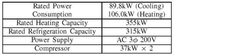
Fig. 3 shows the schematic diagram of the whole air conditioning system. The distribution of heat to fan–coil units inside the building is done by hot water. In the heat pump unit, there is a valve that controls the flow of refrigerant. The control of the valve is done via hydraulic system. The heat pump unit has two external terminals that correspond to Load Up and Load Down. Signals given to these terminals control the valve and changes the amount of refrigerant compressed by the compressor. As aresult, the power consumption of heat pump unit changes. The experiment is conducted under heating operation and only one of the two heat pump units is controlled. The error ratio of the measurement system is with in 2%.

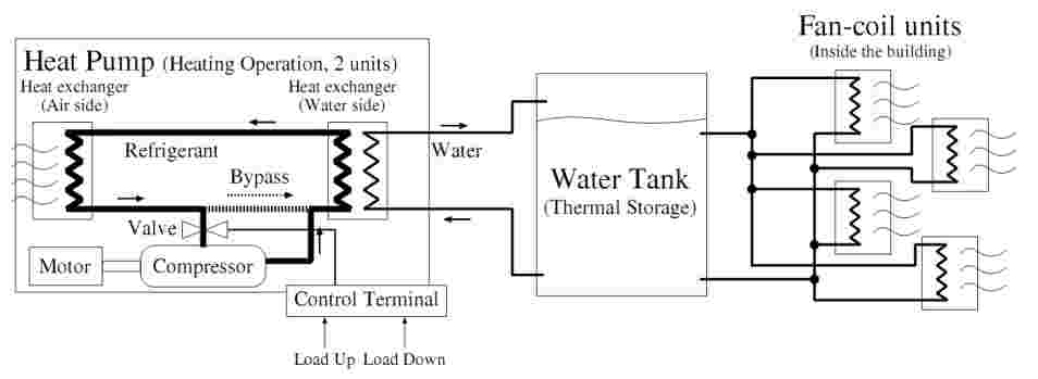
Figure 3 – Air conditioning system used in experiments.

B. Step Response Test.

In the step response test, a simple Load Up or Load Down signal was given to the heat pump unit and change in its power consumption was measured. The experiment was conducted in the following two cases:

Case 1:Power consumption minimum – maximum

Case 2: Power consumption maximum – minimum

Figs. 4 and 5 show the power consumption response characteristics for case 1 and 2, respectively.

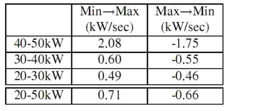
These results show that the heat pump responds quickly when it is heavily loaded. Table III shows the average rate of change of power consumption that is calculated every 10 kw.

The table shows that response speed of power consumption by a rate of change of at least 0.45kW/s can be expected when heat pump is used for power compensation.

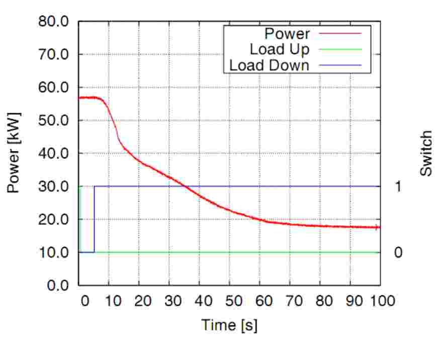
Figure 4 – Step response test (Min to Max)

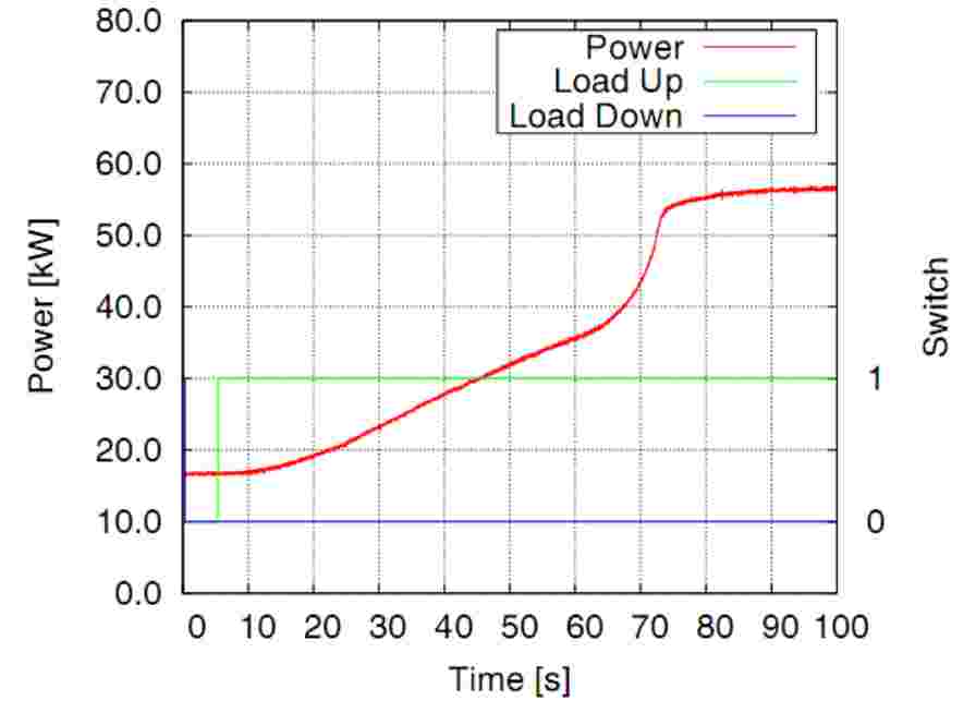
Figure 5 – Step response test (Max to Min)

Table III – Power consumption average rate of change

С. Sinusoidal Wave Response Test.

Sinusoidal wave response test was done to analyze the response characteristic of the heat pump more quantitatively. Also, sinusoidal wave response test is severer test for the heat pump since the reference signal changes continuously.

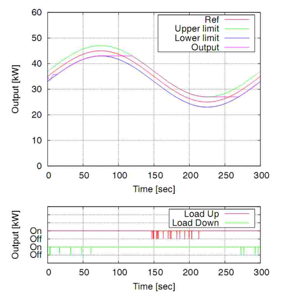
Figure 6 – Example of reference sinusoidal wave

Table IV – Parameters of wave

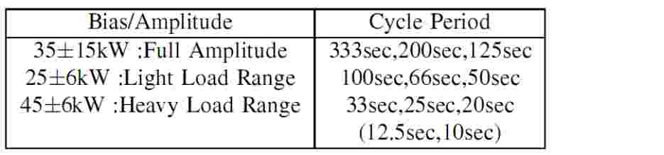
Reference sinusoidal wave was given to the heat pump by changing Load Up and Load Down signal according to the pattern calculated by microcomputer. The pattern was calculated so that the power consumption does

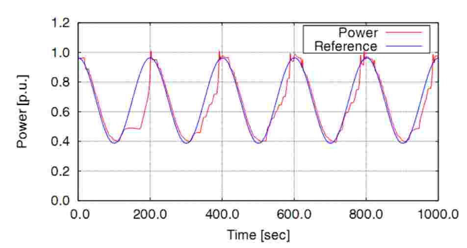
Figure 7 – Sinusoidal wave response (Full Amplitude, 200sec)

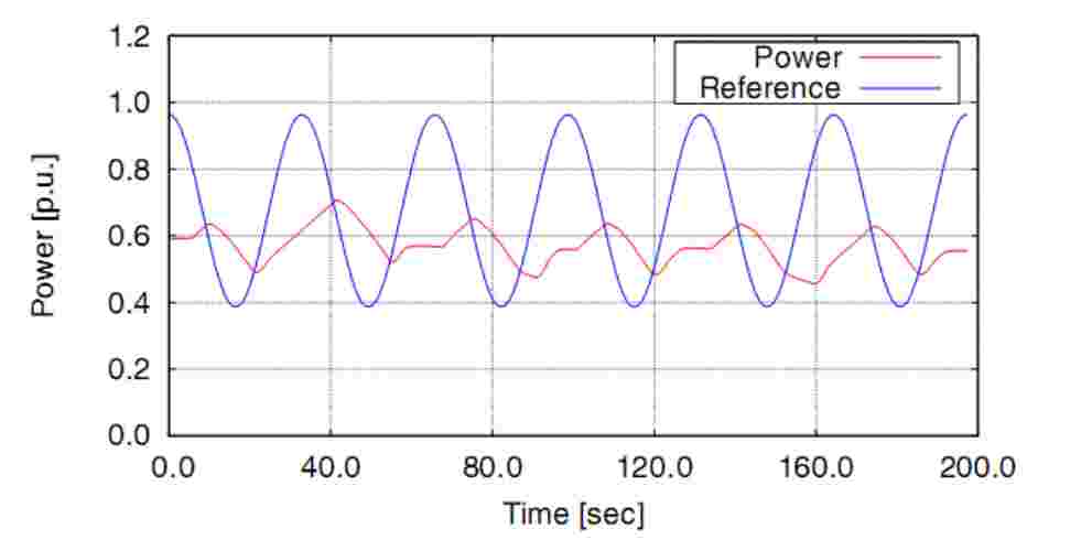
Figure 8 – Sinusoidal wave response (Full Amplitude, 33sec)

Figs. 7 and 8 show typical results of sinusoidal wave response test. In the case of Fig. 7, the power consumption of the heat pump follows its reference signal, but in the case of Fig. 8, the change of reference signal is too fast to follow.

Discrete Fourier transform (DFT) was used to determine the frequency response of power consumption, and phase lag and amplitude plotted as Bode diagram are shownin Fig.9.InFig.9, three Bodediagram sare plotted based on three amplitude range test conducted in sinusoidal wave response measurement: full amplitude range, heavy load range and light load range. In Fig. 10, the frequency response of the heat pump is compared with those of other apparatuses: NiMH battery, electric double layer capacitor(EDLC), and gas engine.

Table V – Minimum sinusoidal wave period that power consumption can follow

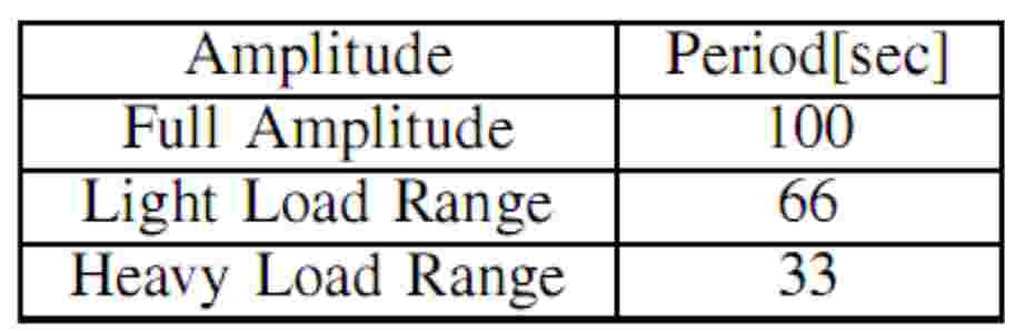
Table V shows the minimum period of sinusoidal wave that the power consumption can follow when -3dB is considered as the border value.

The heat pump’s frequency response is faster than that of GE and slower than those of ESSs when heat pump is operated in heavy load range. Thus, the control of the heat pump can compensate faster power fluctuation compared to the GE and has possibility of reducing the necessary energy capacity of ESSs.

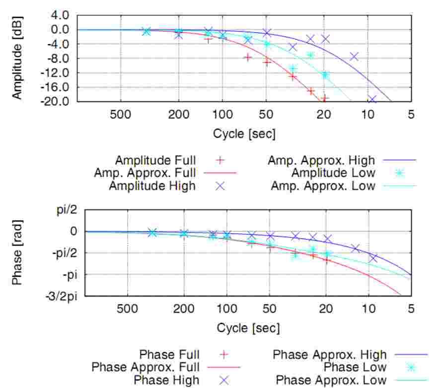
Figure 9 –Bode diagram (Above:Amplitude, Below:Phase)

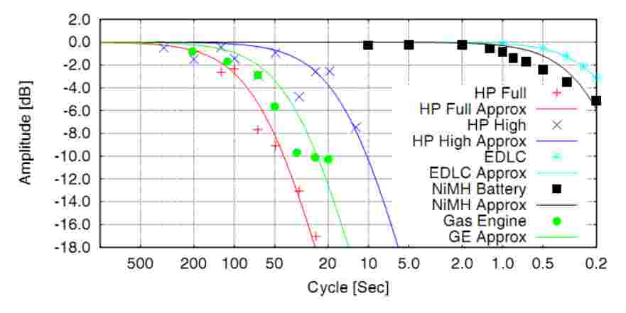
Figure 10 – Comparison with response of other apparatuses

III. Microgrid control simulation including heat pump

Based on the result obtained from the experiment, a microgrid control simulation including heat pump air conditioning system was carried out.

А. Model Microgrid.

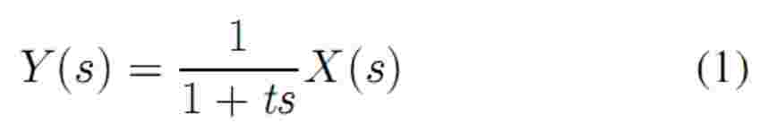
A model microgrid with a gas engine(GE), an ESS, and a heat pump is assumed in the simulation. In this simulation, the power consumption characteristic of the heat pump is modeled using a first order transfer function which is represented by (1) in the Laplace domain. Y(s) – is the power consumption, X(s) – is the reference value and t is the time constant of the model. s – indicates the differential operator.

Based on the measured power consumption characteristic shown in Section II, the time constant of the heat pump was set to 30 seconds.

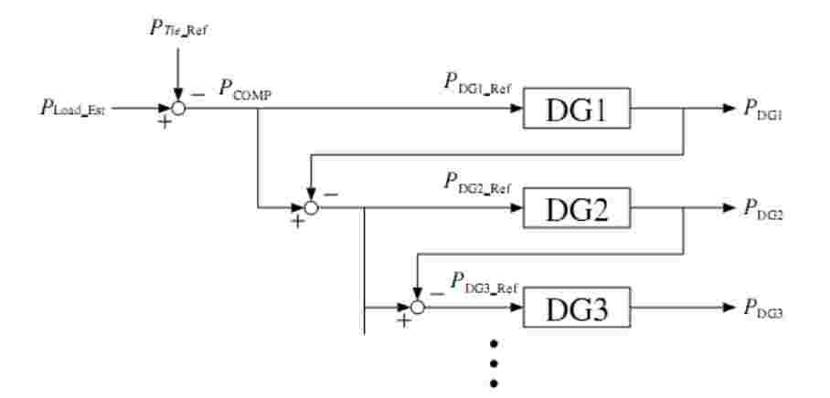
Figure 11 – СBlock Diagram of Cascade Control

The first order transfer function model that is represented by (1) is also used for models of ESS and GE. For ESS and GE, the time constant of the model is 0.04 seconds and 70 seconds respectively.

In this simulation, the state of charge (SoC) of the ESS is calculated by integrating sum of its output and loss during charge and discharge.

As loads in the microgrid, data of the real load is used. In this simulation, the microgrid is connected to the commercial grid via a tie line and the control system is designed to keep the tie line power flow at constant value.

В. Control System

The hybrid control system is used to control the power of the GE, ESS, and heat pump. This control system is a combination of cascade control and local control[4].

Fig. 11 shows the block diagram of the cascade control system. In the cascade control, the power consumption within the microgrid is estimated by measuring the tie line power flow and output power of DGs. The amount of power that needs to be compensated (P_COMP) is calculated by subtracting the reference value of the tie line power flow from the estimated load. As shown in Fig. 11, the DGs in the microgrid are organized according to their active power output response speed. The DGs that have a slower response compensates the power first and the remaining P_COMP is compensated by the faster DGs. When ESSs are used for compensation, their state of charge(SoC) is controlled by sending the SoC signal to slower DG.

The block diagram of the control system used in the simulation is shown in Fig. 12. The part drawn in red lines is the control system of the heat pump.

The reference signal of the GE is put through an LPF with a time constant of 200 seconds to prevent the GE from fluctuating too fast. Furthermore, to prevent excess compensation of the ESS's SoC, the SoC signal is put through an LPF with a time constant of 100 seconds.

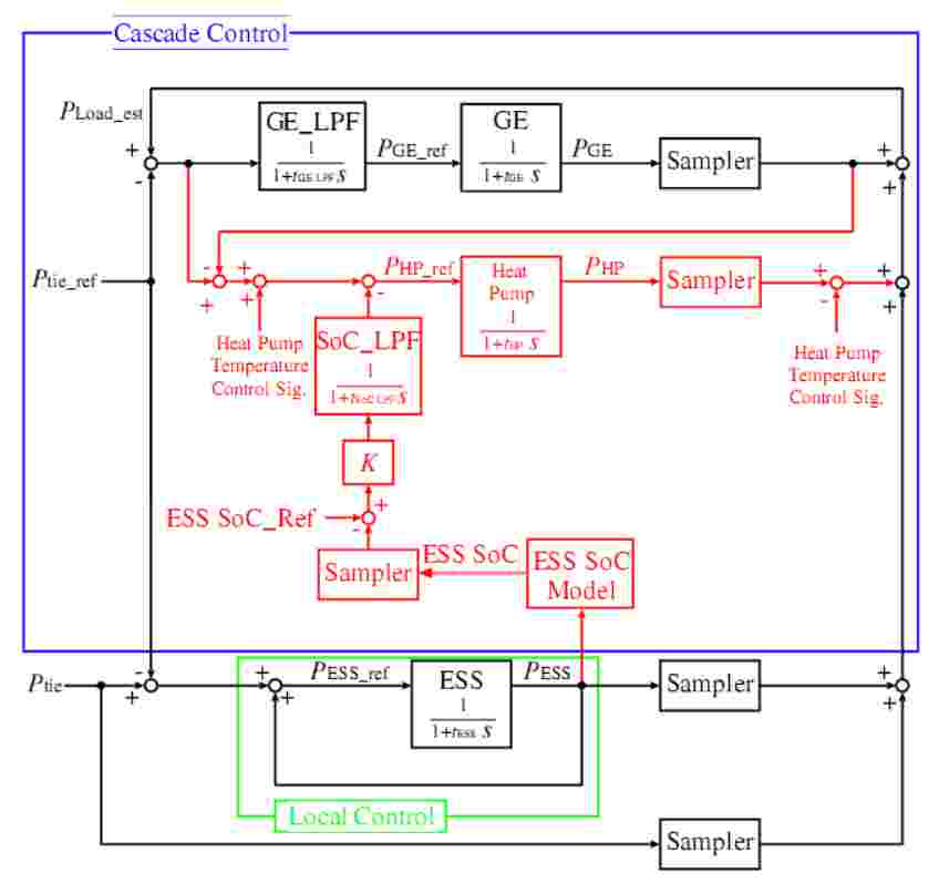
Figure 12 – Block Diagram of Control System in Simulation

C. Temperature Simulation and Control

To study the effect of the heat pump control, a temperature simulation of the space inside a building was carried out at the same time. The temperature was calculated based on heat balance of the room which is shown in Fig. 13. Assumed size of the room is 3 x 5 x 5 = 75 [м³] and assumed size of the window is 2 x 4=8 [м²].

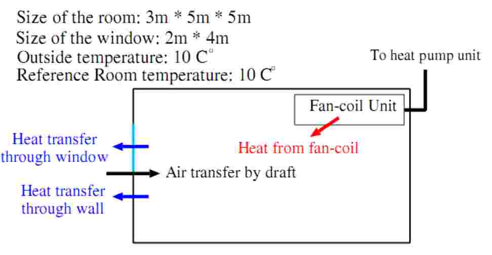
Figure 13 – Heat Balance of Room

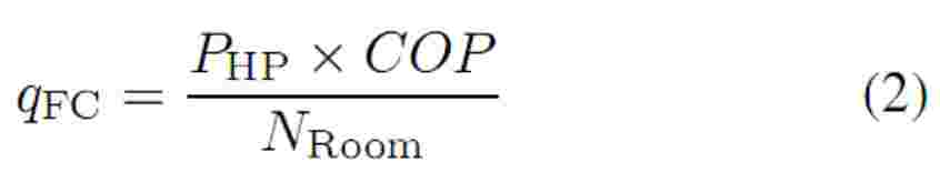
Heat from the fan–coil unit (q_fc [W]) is calculated by (2) [3]. In (2), P_HP[W] is the power consumption of the heat pump unit, COP is the coefficient of performance of the heat pump, and N_Room is number of the rooms to be heated. In this simulation, the value of COP is 2.5. The value of N_Room is 200 which is roughly equivalent to area that the heat pump system used in the experiment covers.

Heat flow through the wall (q_out[W]) is calculated by (3) [7]. A_W [m²] is the area of wall, K_W [W / (m² · К)] is the heat transfer coefficient of the wall, T_room is the room temperature, and T_out is the outside temperature. When concrete wall 150 millimeters thick is assumed, the value of K_W is 3.81[W/(m² · K)].

Heat flow through the window can also be calculated by (3), but the value of K_W is different from that for concrete wall. When glass window is assumed, the value of K_W is 6.4[W/(m² · K)].

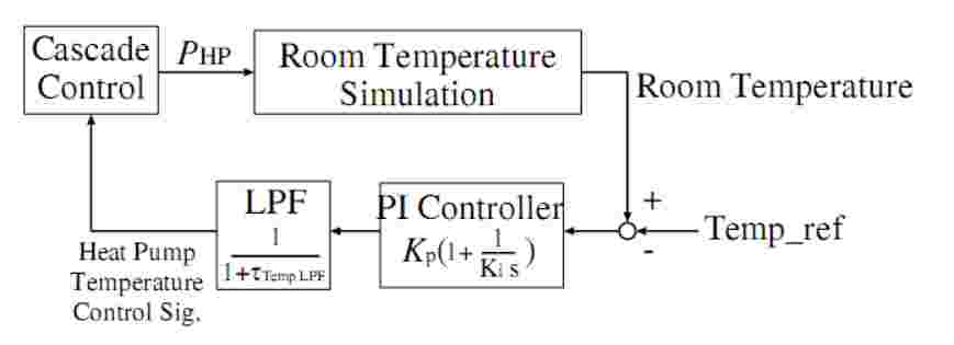
Figure 14 – Temperature Control

Table VI – Simulation cases

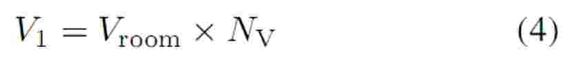
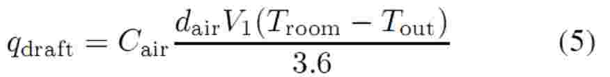
The effect of draft through small gaps in the wall is taken into account by calculating the air volume of the draft (V₁[m3]) which is calculated by (4). In (4), V_room is the volume of the room, and N_V[times/hr] is frequency of ventilation caused by draft. For middle-grade buildings, value of N_V is about 1.0[times/hr].

After calculating V₁, the heat loss by draft (q_draft [W]) can be calculated as shown in (5), where d_air is air density, and C_air is specific heat of air.

In the simulation, the reference room temperature is set at 25 °С, and outside temperature is set at 10 °С.

The Heat Pump Temperature Control Signal in Fig.12 is calculated so that the room temperature would remain at a constant value. Fig. 14 shows the control loop of the temperature. Parameter K_p, and K_i is 50 and 100 respectively. The time constant t_TempLPF is 2 seconds.

D. Simulation Result

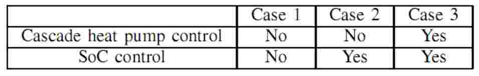
The simulations were carried out for three cases shown in Table VI.

In case 1, the heat pump operates only according to the temperature control and the SoC of the ESS is not controlled. In case 2, the heat pump operates only according to the temperature control, but the SoC of the ESS is controlled by the GE. In case 3, the heat pump operates according to the cascade control and the temperature control, and the heat pump, which has faster response characteristic compared to the GE, controls the SoC of the ESS.

Fig. 17 shows the outputs of the DGs and power consumption of the heat pump for the three cases. Fig. 15 shows the SoC of the ESS and Fig. 16 shows the change in room temperature. The value 0 kWh in Fig. 15 indicates initial value of SoC. In Fig. 16, the line of case 2 overlaps the line of case 1 almost completely.

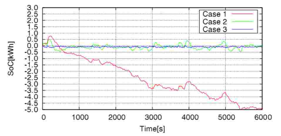
Figure 15 – SoC of the ESS

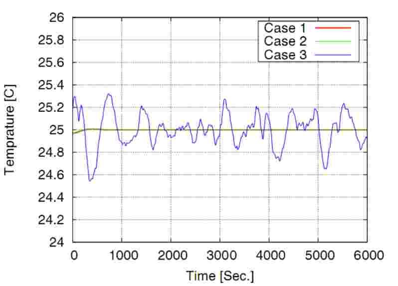
Figure 16 – Room temperature

Table VII – Statistical figures of tie line power flow

Compared to case 1 and 2, the fluctuation of the ESS’s SoC is suppressed in a narrow range in case 3. On the other hand, there is a large fluctuation of the room temperature in case 3. There was no significant difference in tie line power flow between three cases as shown in TableVII. A summary of results that consists of SoC data and building temperature are given in Tables VIII and IX.

These figures indicate that the control of the heat pump suppresses energy fluctuation of the ESS. Instead, fluctuations in the building temperature increase.

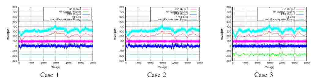
Figure 17 – Output of DGs and power consumption of the heat pump

Table VIII –Statistical figures of SoC data

Table IX –Statistical figures of room temperature

IV. Conclusion.

Heat pump air conditioner have long time constant against disturbance. Thus, control of heat pump in a microgrid seems to be an effective method to reduce the ESS’s energy capacity required to compensate power fluctuations without affecting the room temperature significantly.

In this paper, the step response and sinusoidal wave response characteristics of a heat pump’s power consumption were measured experimentally as a case study. It was verfied that power consumption of heat pump can follow sinusoidal wave whose period is 33 seconds or longer.

Using the characteristic derived from the experiment, a simulation of microgrid control including heat pump control was carried out. The result showed that the heat pump control is effective to reduce the energy capacity of ESS, with relatively small change to the room temperature.

References

1. S. Kawachi et al. Energy Capacity Reduction of Energy Storage System in Microgrid Stabilized by Cascade Control System EPE2009, Barcelona, Spain, No.0208, September 2009
2. H. Irie, A. Yokoyama, Y. Tada Modeling for Frequency Control Analysis of Power System with a Large Penetration of Wind Power Generation by a Lot of Controllable Heat Pump Systems and Battery Systems, POWERCON 2008 & Power Conference in India, 0455, Delihi, India, 2008
3.W. Giedt Principles of Engineering Heat Transfer D. VAN NOSTRAND CO., Inc., New York, 1957
4. T. Kikuchi et al. High Quality Power Supply Method for Islanding Microgrid by use of Several Types of DG Systems including Rotation Machines IEEJ Trans. Power & Energy, Vol.129, No.12, pp1561-1566, 2007 [In Japanese]
5. Electric Technology Research Association Report Vol.56 No.4 Technology of Distributed Power Source and Prospective View of Power Network, 2001 [In Japanese]
6. Y. Nishizaki Blade Pitch Angle Control and its Capacity Reduction Effect on Battery for Load Frequency Control in PowerSystem with a Large Capacity of Wind Power Generation IEEJ Trans. PE, Vol.129, No.1, 2009 [In Japanese]
7. Japan Society of Refrigerating and Air Conditioning Engineers Standard Elementary Text -Refrigeration and Air Conditioning Technology-, 2009 [In Japanese]