Abstract— This paper presents an analysis of the alg orithms used for generating 3D structures from 2D CT-Scan Datasets. This is achieved by developing an implementation of Marching Cubes, a surface construction algorithm that’s currently the standard used for 3D surface construction in the medical visualization industry. Two techniques have been chosen to produce the 3D models. The first technique is known as Volume Rendering and the second technique is known as the Marching Cubes Algorithm. Both techniques use voxels (3D square pixels) to determine the 3D area to be constructed. The Marching Cubes (MC) algorithm by Lorensen and Cline is most popular algorithm for extraction of isosurface out of volume data. Several drawbacks of MC algorithm are solved by using new improved version of MC algorithm.

Index Terms— Marching Cube, 3D surface reconstructio n, isosurafce, Volume rendering, Medical imaging

I. INTRODUCTION

X-ray Computed Tomography (CT) is a medical imaging technology used by doctors to diagnose areas of interest within the body non-invasively. CT-Scans of patients are generated by having an X-ray source that rotates around a patient; X-ray sensors are positioned on the opposite side of the circle from the X-ray source. Many data scans are progressively taken as the object is gradually passed through the gantry. They are combined together by the mathematical procedure known as tomographic reconstruction [9, 10, 11], which generates two-dimensional (2D) images that doctors use when diagnosing patients. Yet 2D images cannot accurately convey the complexities of human anatomy. Interpretation of 2D complex anatomy requires special training and though radiologists are trained to interpret these images, they often find themselves having to communicate their interpretations to a physician, who may have difficulty imagining the three-dimensional (3D) anatomy [3]. However, this same anatomy can be visualized as a 3D image, allowing doctors to properly see the volume and shape of features that they may be interested in analyzing, such as the brachial tree, a particular tumor or other features of interest.

The Marching Cubes (MC) algorithm by Lorensen and Cline [1] is the most popular algorithm for the extraction of isosurface out of volume data. We propose a robust and intelligent triangulation strategy and performing complementary and rotational symmetry operation. This is a significant practical improvement compared to the former scheme of isosurface tilings. The 3D images are developed from 2D CT/MRI scans of a particular object of interest. The core of this algorithm is the creation of 3D CT/MRI rendering software. The software will produce a 3D interpretation of 2D CT/MRI data. Initially, the software stacks the 2D data to form a large cube of data. Statistical classification is used to create and label voxels (3D pixels).

Manuscript received on June, 2013.

Pravin P Kalyankar, Department Of CSE, Dr.BAMU Aurangabad.TPCT COE osmanabad, Indiaity, India.

Dr.S S Apte, WIT Solapur, Department of CSE, Solapur University/ India.

Finally, the Marching Cubes algorithm is used to extract and create polygon surfaces from the volume. Some limited user interaction is permitted such as rotating, scaling and moving the volume.

II. CT-SCAN ACQUISITION FOR 3D VISUALIZATION

In order for any 3D surface reconstruction algorithm to properly work, it is important to address the special considerations required of the set of slices for the algorithm to work. Of the different concerns that are normally under consideration for X-Ray CT – fan-beam reconstructio n, spiral/helical CT, multi-slice spiral CT – very few directly affect the nature of the 3D structures that are produced. As long as the 2D slices have the same resolution, spatial orientation, and are stored sequentially, then the 3D visualization should generate an accurate representation. It is important for each image to have the same resolution because the algorithm assumes that corresponding pixels in each slice will correspond to the next pixel value in that same physical direction. Similarly, if the spatial orientation of the images is different (rotated, flipped, etc.) then corresponding pixels in different slices will not generate an accurate not accurately represent the continuous space in which the dataset was captured, the visualized structure will be inaccurate. For example, if the first half of a set of slices taken of the head and torso was mistakenly placed behind the second half, the structure would appear to have the head attached to the bottom of the torso. However, as long as these conditions are met, any algorithm used will produce structures that accurately represent the imaged space.

III. RENDERING 3D SURFACES

Currently, there are two general models used for rendering 3D images. The first is known as Volume Rendering and the second is known as the Marching Cubes Algorithm. Both use voxels (3D square pixels) to determine the 3D area to be constructed. The Marching Cubes (MC) algorithm by Lorensen and Cline is most popular algorithm for extraction of isosurface out of volume data. Our algorithm is adaptive to the small the changes of data or the small changes of the threshold, and obtains more reasonable result of triangulation of isosurface than those produced by standard MC algorithm. Marching Cubes Algorithm is considered a thresholding technique because it uses only the pixel information at the eight corners of the voxel.

IV. MARCHING CUBES ALGORITHM

The current standard algorithm for 3D surface construction is the Marching Cubes algorithm, methods of 3D surface construction. The algorithm implements threshold rendering in order to generate “triangle models of constant d ensity surfaces from 3D medical data” [4]. In summary m arching cubes creates a surface from a three dimensional set of data as follows:

1.Read four slices into memory.

2.Scan two slices and create a cube from four neighbours on one slice and four neighbours on next slice.

3.Calculate an index for the cube by comparing the density values at the vertices with surface constant.

4.Using the index, look up the list of edges from pre- calculated table.

5.Find the surface–edge intersection via linear interpolation.

6.Calculate a unit normal at each cube vertex and interpolate the normal to each triangle vertex.

7.Output the triangle vertices and vertex normals. Subsequently, linear interpolation is performed to obtain the coordinate of the intersected point. This is done through the formula below:

P=P1+ ((T-V1) / (V2-V1))*(P2-P1)	(1)
where
T = threshold value used to identify isosurface
P = coordinate of the intersected point
P1, P2 = coordinate of the vertices of the intersected edge
V1, V2 = scalar values at each vertex

Gradient Calculations are used to estimate the normals of the triangle vertices. This is done by estimating the gradient vectors at the point of intersection. Given a voxel at (i, j, k) the gradient is estimated using central differences along the 3 co-ordinates axes by:

Gx (i, j, k) = D (i+1, j, k) - D (i-1, j, k)/ length(x)
Gy (i, j, k) = D (i, j+1, k) - D (i, j-1, k)/ length(y)
Gz (i, j, k) = D (i, j, k+1) - D (i, j, k-1)/ length (z)	(2)

Where D (i, j, k) is the density function (RGB value) at pixel (i, j) in slice k and length(x), (y), (z) are the lengths of the cube edges.

V. ONE CUBE

At the basic level, the Marching Cubes algorithm takes eight scalar values from two adjacent slices of our dataset to form the vertices of an imaginary cube. After establishing our imaginary cube, we compare the value of a single vertex of our imaginary cube against some desired value, also known as an isovalue. If the value of the vertex is less than or equal to our isovalue, we can then say it falls within (or on) the surface. Otherwise, it falls outside the surface. We repeat this operation with the other 7 vertices to determine which points are inside or outside the surface we want to render. Once we determine which parts of the cube fall within the desired surface, we then create a topology of the surface within the cube [4].Because there are eight vertices per cube and only two logical states (inside or outside) per vertex, there are 256 ways a surface can intersect a single cube. While triangulating the 256 possibilities for each imaginary cube is feasible, this is not recommended because triangulating the 256 possibilities tends to be tedious and error-prone [4]. For example, the topology of a triangulated surface remains the same when the relationships of the surface values are inverted [4]. This reduces the number of possible cases from 256 to 128. Also, because there’s rotational symmetry within some of the 128 cases, we can reduce the number of analyzed cases from 128 to 14, and rotate the appropriate case when necessary. Figure 1 shows the triangulation for 14 cases. By just analyzing 8 vertex values, we can generate a precise surface that can be expressed as a combination of 5 or less triangles.

Figure 1: Triangulated Cubes

VI. MULTIPLE CUBES

When applying the algorithm to multiple cubes, the same approach is taken for each individual cube as described in the previous section. Looping through the cube space, one cube at a time, triangles are calculated for each. However, it is important to note that the relationship between cubes is that every cube shares 4 vertices with each cube adjacent to it [4].This is shown in Figure2 where the vertices 0, 1, 2, and 3 touch both cubes.

Figure 2: Adjacent marching cubes with connected isosurface

In this way, cubes are connected to each other because their vertices are overlapped. This ensures that calculating one cube at a time will result in the creation of the same surface regardless of the order in which cubes are traversed. In Figure 2, this concept can be seen taking shape as the two surfaces in each cube are connected at their shared face. In order to view different structures within slices, one changes the isovalue parameter of the algorithm. This effectively tells the algorithm to create polygons out of a different range of pixel values.

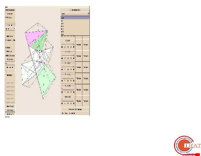
Figure3 shows the interface of the applet. This applet is supposed to give the visitor the opportunity to view the marching cubes algorithm running on different cases, and experiment with it. Here is the list of the operations the user is able to perform:

1)Modify the weight of vertices:

To achieve this goal, the user must select the cube he wants

to change using a combo box or space key, which cycles through all existing cubes. Then he has choose and modify the vertex of selected cube using slider bars.

2)View the cubes from any angle:

User is able to control the viewport by rotating or

translating the object of the scene.

3)Build a mesh with different cubes:

It is possible to add or delete cubes. To add a cube the user

only has to select an existing one and pick one of his face and click the appropriate button: a new cube will be added using the specified face and vertices connected to other cubes will be merged with them.

4)Choose ambiguous and complementary cases.

Ambiguous cases can generate holes in the computed

isosurface, modifying the view provides a useful tool to keep correct topology.

5)Control rendering parameters.

Rendering parameters describe the aspect of the objects in

the scene like colour, shininess. Many materials like ruby, jade and two lighting models are available to let the user to customize the visualization.

The pseudo-code looks like this: if (resolve ambiguous cases)

draw(TrianglesA[15*cube]); else

if (cube belongs to Ambiguous) draw(reverseNormals(TrianglesA(255-15*cube)));

else draw(TrianglesA[15*cube]);

VII. LOOKUP TABLE

To speed up the Marching Cubes algorithm, we created an index to an array that has pre-calculated each of the 256 possible surface intersection configurations. We then assign the scalar value of each vertex a bit in an 8-bit integer. If the vertex’s value falls within the range of our isovalue, we then set the corresponding bit to 1. Otherwise the same bit is set to 0. The final value of this 8-bit integer is the corresponding surface intersection configuration. For each on-off combination of the cell vertices (there are 256 different combinations), the standard lookup (lut) table codes the number of triangles produced and the cell edges on which these vertices lie.

Following lookup tables are implemented.

1)Ambiguous.lut.txt: It contains the numbers of cases whose complementary is changed when solving topology problems.

2)TrianglesS.lut.txt: It contains the indexes of interpolated vertices to draw when using standard complementary cases

3)TrianglesA.lut.txt: It contains the indexes of interpolated vertices to draw when using ambiguous complementary cases.

VIII. CONCLUSION

Visualization of medical data in 3D is a valuable tool that will assist physicians in diagnosing and treating patients with greater confidence. By using algorithms such as Marching Cubes, such visualizations can be generated with relative ease. Improvements in the graphical capabilities of computers and the optimizations of existing implementations of this algorithm will increase the visibility of such visualizations in regular medical practice.

REFERENCES

[1]Bourke, P. “Polygonizing a Scalar Field”, May 1 994, http://astronomy.swin.edu.au/~pbourke/modelling/polygonise/

[2]Cline, H., Lorensen, W., System and Method for the Display of Surface Structures Contained Within the Interior Region of a Solid Body, US Patent 4,710,876, to General Electric Corp., Patent and Trademark Office, 1985

[3]Dedual, N., Kaeli, D., Johnson, B., Chen, G., Wolfgang, J., “Visualization of 4D Computed Tomography Datasets”, Proc. 2006 IEEE Southwest Symposium of Image Analysis and Interpretation, March 2006

[4]Lorensen, W., Cline, H. “Marching Cubes: A Hig h Resolution 3D Surface Construction Algorithm”, ACM Computer Graphics Volume 21, Number 4, July 1987

[5]Johnson, C., Parker, S., Hansen, C., Kindlmann, G., and Livnat, Y. “Interactive Simulation and Visualization” Center for Scientific Computing and Imaging, University of Utah. http://www.cs.utah.edu/sci

[6]Keppel, E. “Approximating Complex Surfaces by Triangulation of Contour Lines” IBM J. Res. Develop 19, 1 (January 1975), p. 2-1

[7]Robb, R. A., Hoffman, E. A., Sinak, L. J., Harris, L. D., and Ritman, E. L. “High Speed Three-Dimensional X-Ray Computed Tomography: The Dynamic Spiral Reconstructor”, Proc. Of IEEE 71, 3 (March 1983), 308-319.

[8]Sabella, P. “ A Rendering Algorithm for Visuali zing 3D Scalar Fields” ACM Computer Graphics Volume 22, Number 4, August 1988

[9]Webb, A. Introduction to Biomedical Imaging, Wiley-Interscience, 2003, p. 34 - 47

[10]“Computed Tomography” , Wikipedia, 17 April 2006, http://en.wikipedia.org/wiki/Computed_Tomography

[11]“Tomographic Reconstruction”, Wikipedia, 24 March 2006, http://en.wikipedia.org/wiki/Tomographic-reconstruction