Abstract

The volume rendering is one of the most useful techniques in medical visualizations, computer-aid diagnosis and other related areas. Among all the different approaches to realize it, the marching cube algorithm is the most popular one. This report is to present our approach to implement this algorithm. According to the algorithm, the whole volume data is divide into small cubes, each of them contains image data on the eight corners. The next step is to construct triangular patches on the isosurface by checking the cubes corners with the user- specified isovalue. By connecting the patches, a 3D model is represented.

1. Introduction

In medical image processing, re-assembling a three-dimensional model from a set of CT- scan or MRI-scan is very attractive to medical workers. The 3D model is much helpful for physicians to understand the inner anatomy of patients than the 2D slices. The visualizations also helps in the communication. Among all the different approaches to realize it, the marching cube algorithm[1] is the most popular one.

Marching cube algorithm can produce high quality image result so that doctors can analyze organ or other part of the body. More conveniently, the algorithm can re-

jiny@usc.edu xuxinche@usc.edu

assemble the three dimensional model based on a parameter called iso-level value, which is similar to the definition of depth. In other words, depending on the iso-level, the user can see different depth from skin to organ model assuming the CT-scan is taken from a human body.

After the first paper presenting the marching cube algorithm, many researchers contribute to improve the algorithm in many ways. Some improvements are focus on the correctness by providing more detailed lookup tables[2] [3] and reducing ambiguous[4]. Others are based on efficiency by approximating normals[5] and reducing the triangles[6].

2. Acquisition

Before discussing the algorithm in Sec.3, we will first overview our setup for tools and environment, data collection, and graphical user interface.

Setup for tools and environment For the

purpose of this project, we decided to use some libraries that will make implementation easier. First of all, we decided to make a graphical user interface so that the user can easily load in the volume data and see the rendered result. Since all of us are somewhat familiar with C++, that is an obvious choice for us. In addition, we are using two open-source libraries. One is

OpenGL, which is a popular graphics framework. The other one is Qt, which we exploited a subset to build the user-friendly graphical interface. Luckily, all of these tools and libraries interact very nicely together in Visual Studio 2008.

Graphical user interface We created a

user-friendly graphical user interface for executing the program. The GUI is used mainly used for loading the volume data into the underlying data structure and those data will be fed into the marching cubes algorithm. The GUI also allows the user to set iso-level and resolution easily so that user can adjust different parameters. Most importantly, the GUI has a view outlet to display the triangles produced from the marching cubes algorithm. Overall, we try to make the GUI easy to use.

3. Marching Cubes Algorithm

The graphics algorithm we use is called marching cubes algorithm. Lorensen and Cline first published it in 1987. This algorithm produces a triangle mesh by computing iso-surfaces from discrete data. By drawing all these triangles, we can build a three dimensional representation of the CT-Scans.

The marching cube algorithm can be divided into two main parts. The first part is to figure out how to define the sections of surface that cut up an individual cube. There are a total of 256 possible configurations of corner classifications if we classify each corner as either being below or above the isovalue. In these 256 possible configurations, two of them are trivial. They are the cases where all points are inside or

outside the cube, which does not contribute to the isosurface. For the rest of the configurations, we have to decide whether the isosurface crosses along each cube edge, and use these edge intersection points to construct one or more triangular patches for the isosurface. We assign 0 to vertex outside the surface and assign 1 to vertex inside the surface. (Figure 1)

When symmetries cases are considered (Figure 3), there are only 14 unique configurations in the rest of the 254 configurations indeed (Figure 4). In the case that only one corner is less than the isovalue, it forms a single triangle which intersects the edges which meet at this corner, with the patch normal facing away from the corner. There are 8 similar configurations belongs to this case. We should calculate an index for the cube by comparing the eight density values at the cube vertices with the surface constant. (Figure 5). We can get 8 configurations which have 7 corners less than isovalue by flipping the normal, and they are not unique. For those configurations that have 2 corners less than the isovalue, there are 3 unique configurations, regarding whether the corners belong to the same edge, same surface of the cube, or are diagonally positioned relative to each other. For those configurations with 3 corners less than the isovalue, there are 3 unique configurations depending on whether there are 0, 1, or 2 shared edges that form an “L” shape. When there are 4 corners less than the isovalue, there are 7 unique configurations depending on whether there are 0, 2, 3, or 4 shared edges.

There are between 1 and 4 triangles being added to the isosurface for each of the non- trivial configurations. Interpolation along edges can be used to compute the actual vertices. Another way to compute the actual vertices is to default their location to the middle of the edge. But the interpolated locations will give a better shading calculations and smoother surfaces.

to the whole volume. Volume can be processed in slabs, where each slab is consists of 2 slices of pixels. Each cube can be treated independently or propagate edge intersections between cubes which share the edges. Another option to do this sharing is between adjacent slabs, this will increase storage and complexity a bit but the advantage is less computation time. The sharing of edge and vertex information also results in a more compact model, and one that is more amenable to interpolated shading.

Figure 1.

Figure 2 Triangulate each case

Figure 3

Now we are able to create surface patches for a single voxel, which by can be applied

Figure 4

Figure 5

The final step in marching cubes is to calculate a unit normal for each triangle vertex. It is used to create Gouraud-shaded

images in the rendering algorithms. Interpolate the normal to each triangle vertex and output the triangle vertices and vertex normals.

4.Equation

∙Interpolate surface intersection along each edge

∙Calculate normal for each cube vertex:

∙Interpolate the normals at the vertices of the triangles:

5. Implementation

The concept of the marching cubes algorithm was explained in the last sections. To realize this algorithm, there are a few more data structures we have to define. The first one is a coordinate “XYZ” class in which it will have the x, y and z coordinate of one vertex. The second one is the Triangle class in which in it will have three

“XYZ” objects. The third one is the Grid Cell class in which it will contain 8 “XYZ” objects for 8 vertices and their corresponding iso-values.

Out of the three data structures, perhaps the Grid Cell is the most interesting one. It is used to store the ISO values at each of the 8 vertices. Assuming we are running marching cubes algorithm on every pixel, 256 of these cubes will be created for every two slices of images if each image has 256 by 256 pixels and we make a cube per pixel.

After the cube for a pixel is constructed, we need to identify which vertex is below the iso-surface. To do that, we have to evaluate the iso-value for each vertex. We use a bit vector (cube index) to record those vertices that are below specific iso-value.

There are 256 of possible combinations of how the edges of a cube are intersected by the iso-surface. We use an array of hexadecimals to store all 256 different possibilities. This is called edge-table.

Similar to what we did for edge table, again a table is used which this time uses the same cube index but allows the vertex sequence to be looked up for as many triangular facets are necessary to present the iso-surface within the grid cell. This is called tri-table.

I will give an example using the combination of the above data structures. For example, after we construct the cube, we find out that vertex 0 and vertex 3 are below the iso-value. The cube index will be

“00001001”, which is 9. We use this cube index, 9, to look up the edge table. We then get 905 in hex, which is equivalent to

“100100000101”. This represents that edge

0, 2, 8, 11 are intersect with the iso-surface. After we identify the edges, we need to do a linear interpolation to calculate the intersection points.

P = P1 + (iso-level – V1)(P2 – P1)/(V2 – V1)

Then we know a particular point on the edge that intersects with the iso-surface. The last thing we need to do so to farm the correct facets from the positions that the iso-surface intersects the edges of the grid cell. Using the same cube index, we will go to the tri- table to look up the triangle information.

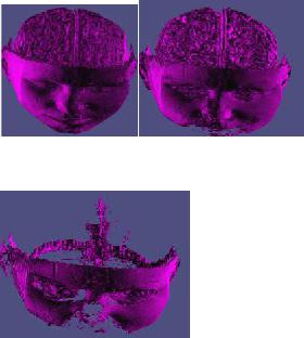
Finally, we need to calculate the normal vectors for each triangle. In order to do this, we first calculate normal values on each node of the cube based on the gradient method, and then interpolate the triangle vertex normal. With the calculated normal vectors, we could do gouraud shading on the constructed 3d model, which made the output looks much better with flat shading.

6. Difficulties

First of all, we selected two different libraries which none of us have ever used before, which is Qt and OpenGL. A lot of efforts were put in to understanding of how to use these libraries correctly. Luckily, Qt has support for OpenGL although not much. Nevertheless, it makes displaying the result triangles produced by marching cubes algorithm simpler. One interesting thing is that we spent four hours to compile the Qt library. That was both unexpected and time consuming.

However, we have spent more time dealing with OpenGL. Having no knowledge in OpenGL, we have to learn from drawing the basic primitive. In particular, the one function we most care the most about is to draw triangles on the view port.

The second difficulty we had was the availability of the data. It was not easy to find volume data, as it is somewhat private information no one would freely share on the Internet. Luckily, we eventually find it in a volume data archive from Stanford University website. The data we got was in binary format. They are all 16-bit integers. We had trouble verifying the correctness of the data until we draw it on the screen and nothing else to compare to.

The rest of the difficulties we have were related to the marching cubes algorithm. After having the basic knowledge about marching cubes algorithm from lecture, we start reading research paper about marching cubes algorithm. The first research paper about marching cubes is in 1987 by Lorensen and Cline. Research paper is very hard to read, so we have to do a lot of

research on the Internet in order to understand the whole algorithm.

Before starting our implementation for marching cubes algorithm, we have to decide what data structure we should use. The simplest way is to construct a cube structure with 8 vertices, each vertex defined by x, y, z coordinates. But the trade-off for this easy implementation is to have data redundancies. When more than two cubes are drawn side by side, the interconnected edge and vertices are overlapped. This creates re-computation over and over again. Nevertheless, we decided to keep it this way because it is simple and easier to understand.

It really took us a while to realize that we need to process two images at a time to create a cube. We did not understand how to make a cube because we did not understand the relationship between two adjacent CT- Scans.

Not being proficient in C++, our first version had many performance issues. We ended up having to do a lot of profiling on different part of the code. The biggest issue we encountered was that we were making too much unnecessary data copy in between function calls. We spend one whole day just for performance tuning. We are able to increase performance by getting rid of redundant data and passing parameters by reference where possible.

There is another way to increase performance. We can sacrifice some resolution in favor of speed. For example, the default cube size value for the marching cubes algorithm is the same as the number of pixels for the image slice and the default

iso-value is 200. These two default values causes marching cubes algorithm to generate many triangles for our data set. The cube size value is proportional to speed. If we make the cube size to be 4, it will run 4 times as fast as compare to cube size value of 1.

It had been very hard to debug the program. First of all, we were not sure if we had imported the data from the CT-Scan correctly. In fact, we could not even tell the correctness of the algorithm until we see the output. We had done many modifications to the code so that the output would look promising and similar to the CT-Scan.

7. Improvement

There are different ways to enhance the marching cubes algorithm. As explained earlier, in the original paper, there are only 15 different cube configurations, which would lead to ambiguous cases. Ambiguous face is one of the issues that created the topology errors (Figure 6). In Figure 6, we cannot make a decision on the interpretation of this kind of situation. To cope with this problem, we decided to try a different approach proposed by Gregory M. Nielson (reference 5). We basically use a different look up table to represent a set of 22 cube configurations instead of 15 to resolve the ambiguous cases (Figure 7). The new look up table in Neilson‟s paper can resolve the ambiguous cases at the cost of rendering more triangles. In order words, it is slower. We have implemented two different kinds of look up tables, but we decided to keep the look up table that represents 15 different cube configurations in favor of speed.

Figure 7

8. Experiment

We obtained the volume data from Stanford

University‟s volume archive. The files we downloaded from the website contain 16-bit integers in binary format. Those data are read and stored as a vector of 32-bit integers for each slice of images.

We use the following data set for experimenting our tool.

Figure 8-c

Figure 8-d

We test our tools with different isolevels in data set 2. The Figure 9-a, Figure 9-b and Figure 9-c displays the result with isolevels 1500, 2000 and 2500.

Figure 9-c

9. Conclusion

In this report, we are presenting a useful tool implemented by ourself for volume rendering, which could generate a three dimension models from two dimension slice data. Our approach is primarily based on the marching cube algorithm. Although the implementation is time consuming and the debugging is difficult, we finished it on-time and generated the correct result. The result is displayed in OpenGL and QT framework. We did experiment on our tool with Stanford volume data and the result is clear. The demo is available via Youtube <http://tinyurl.com/580demo>

10. Reference

[1]William E. Lorensen, Harvey E. Cline, Marching Cubes: A High Resolution 3D Sur face Construction Algorithm, SIGGRAPH '8 7 Proceedings of the 14th annual conference on Computer graphics and interactive techni ques

[2]Evgeni V. Chernyaev, Marching Cubes 3 3: Construction of Topologically Correct Iso surfaces, 1995

[3]Thomas Lewiner, H‟elio Lopes, Ant‟oni on W „ilsn Vierira, and Geovan Tavares, Eff icient implementation of Marching Cubes‟ c ase with topological guarantees, Journal of Graphics Tools, 2003

[4]Gregory M. Nielson, Bernd Hamann, Th e asymptotic decider: resolving the ambiguit y in marching cubes, VIS '91 Proceedings of the 2nd conference on Visualization '91

[5]Gregory M. Nielson, Adam Huang, Stev e Sylvester, Approximating normals for mar ching cubes applied to locally supported isos urfaces, VIS '02 Proceedings of the conferen ce on Visualization '02

[6]C. Montani, R. Scateni, R. Scopigno, Dis cretized marching cubes, VIS '94 Proceedin gs of the conference on Visualization '94