Abstract
Bilateral filtering smooths images while preserving edges, by means of a nonlinear combination of nearby image values. The method is noniterative, local, and simple. It combines gray levels or colors based on both their geometric closeness and their photometric similarity, and prefers near values to distant values in both domain and range. In contrast with filters that operate on the three bands of a color image separately, a bilateral filter can enforce the perceptual metric underlying the CIE-Lab color space, and smooth colors and preserve edges in a way that is tuned to human perception. Also, in contrast with standard filtering, bilateral filtering produces no phantom colors along edges in color images, and reduces phantom colors where they appear in the original image.
Introduction
Filtering is perhaps the most fundamental operation of image processing and computer vision. In the broadest sense of the term “filtering,” the value of the filtered image at a given location is a function of the values of the input image in a small neighborhood of the same location. In particular, Gaussian low-pass filtering computes a weighted average of pixel values in the neighborhood, in which, the weights decrease with distance from the neighborhood center. Although formal and quantitative explanations of this weightfall-off can be given [11], the intuitionisthat images typically vary slowly over space, so near pixels are likely to have similar values, and it is therefore appropriate to average them together. The noise values that corrupt these nearby pixels are mutually less correlated than the signal values, so noise is averaged away while signal is preserved.
The assumption of slow spatial variations fails at edges, which are consequently blurred by low-pass filtering. Many efforts have been devoted to reducing this undesired effect [1, 2, 3, 4, 5, 6, 7, 8, 9, 10, 12, 13, 14, 15, 17]. How can we prevent averaging across edges, while still averaging within smooth regions? Anisotropic diffusion [12, 14] is a popular answer: local image variation is measured at every point, and pixel values are averaged from neighborhoods whose size and shape depend on local variation. Diffusion methods average over extended regions by solving partial differential equations, and are therefore inherentlyiterative. Iteration may raise issues of stability and, depending on the computational architecture, efficiency. Other approaches are reviewed in section 6.
In this paper, we propose a noniterative scheme for edge preserving smoothing that is noniterative and simple. Although we claims no correlation with neurophysiological observations, we point out that our scheme could be implemented by a single layer of neuron-like devicesthat perform their operation once per image.
Furthermore, our scheme allows explicit enforcement of any desired notion of photometric distance. This is particularly important for filtering color images. If the three bands of color images are filtered separately from one another, colors are corrupted close to image edges. In fact, different bands have different levels of contrast, and they are smoothed differently. Separate smoothing perturbs the balance of colors, and unexpected color combinations appear. Bilateral filters, on the other hand, can operate on the three bands at once, and can be told explicitly, so to speak, which colors are similar and which are not. Only perceptually similar colors are then averaged together, and the artifacts mentioned above disappea.
The idea underlying bilateral filtering is to do in the range of an image what traditional filters do in its domain. Two pixels can be close to one another, that is, occupy nearby spatial location, or they can be similar to one another, that is, have nearby values, possibly in a perceptually meaningful fashion. Closeness refers to vicinity in the domain, similarity to vicinity in the range. Traditional filtering is domain filtering, and enforces closeness by weighing pixel values with coefficients that fall off with distance. Similarly, we define range filtering, which averages image values with weights that decay with dissimilarity. Range filters are nonlinear because their weights depend on image intensity or color. Computationally, they are no more complex than standard nonseparable filters. Most importantly, they preserve edges, as we show in section 4.
Spatial locality is still an essential notion. In fact, we show that range filtering by itself merely distorts an image’s color map. We then combine range and domain filtering, and show that the combination is much more interesting. We denote teh combined filtering as bilateral filtering.
Since bilateral filters assume an explicit notion of distance in the domain and in the range of the image function, they can be applied to any function for which these two distances can be defined. In particular, bilateral filters can be applied to color images just as easily as they are applied to black-and-white ones. The CIE-Lab color space [16] endows the space of colors with a perceptually meaningful measure of color similarity, in which short Euclidean distances correlate strongly with human color discrimination performance [16]. Thus, if we use this metric in our bilateral filter, images are smoothed and edges are preserved in a way that istuned to human performance. Only perceptually similar colors are averaged together, and only perceptually visible edges are preserved.
In the following section, we formalize the notion of bilateral filtering. Section 3 analyzes range filtering in isolation. Sections 4 and 5 show experiments for blackand-white and color images, respectively. Relations with previous work are discussed in section 6, and ideas for further exploration are summarized in section 7.
The idea
A low-pass domain filter applied to image f(x) produces an output image defined as follows
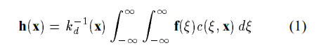
where c(e,x) measures the geometric closeness between the neighborhood center x and a nearby point E. The bold font for f and h emphasizes the fact that both input and output images may be multiband. If low-pass filtering is to preserve the dc component of low-pass signals we obtain.
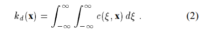
If the filter is shift-invariant, c(e,x) is only a function of the vector difference E- x, and kd is constant. Range filtering is similarly.
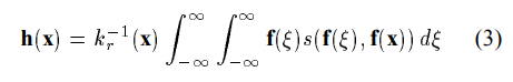
except that now s(f(e),f(s)) measuresthe photometric similarity between the pixel at the neighbo. ood center x and that of a nearby point E. Thus, the similarity function F operates in the range of the image function f, while the closeness function C operates in the domain of f. The normalization constant (2) is replaced by
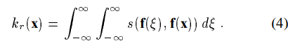
Contrary to what occurs with the closeness function C, the normalization for the similarity function S depends on the image f. We say that the similarity function S is unbiased if it depends only on the difference f(e)-f(x).
The spatial distributionof image intensities plays no role in range filtering taken by itself. Combining intensities from the entire image, however, makes little sense, since image values far away from x ought not to affect the final value at x. In addition, section 3 shows that range filtering by itself merely changes the color map of an image, and is therefore of little use. The appropriate solution is to combine domain and range filtering, thereby enforcing both geometric and photometric locality. Combined filtering can be described as follows
with the normalization
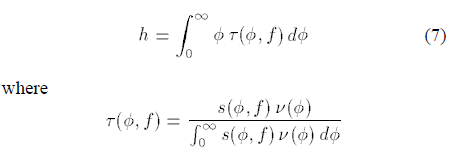
Combined domain and range filtering will be denoted as bilateral filtering. It replaces the pixel value at x with an average of similar and nearby pixel values. In smooth regions, pixel values in a small neighborhood are similar to each other, and the normalized similarity function k^-1 is close to one. As a consequence, the bilateral filter acts essentially as a standard domain filter, and averages away the small, weakly correlated differences between pixel values caused by noise. Consider now a sharp boundary between a dark and a bright region, as in figure 1 (a). When the bilateral filter is centered, say, on a pixel on the bright side of the boundary, the similarity function s assumes values close to one for pixels on the same side, and close to zero for pixels on the dark side. The similarity function is shown in figure 1 (b) for a 23x23 filter support centered two pixels to the right of the step in figure 1 (a). The normalization term k(x)ensures that the weights for all the pixels add up to one. As a result, the filter replaces the bright pixel at the center by an average of the bright pixels in its vicinity, and essentially ignores the dark pixels. Conversely, when the filter is centered on a dark pixel, the bright pixels are ignored instead. Thus, as shown in figure 1 (c), good filtering behavior is achieved at the boundaries, thanks to the domain component of the filter, and crisp edges are preserved at the same time, thanks to the range component.
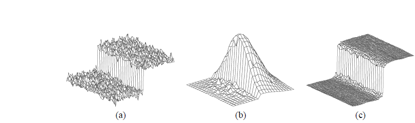
Figure 1: (a) A 100-gray-level step perturbed by Gaussian noise. (b) Combined similary weights for a 23x23 neighborhood centered two pixels to the right of the step in (a). (c) The step in (a) after bilateral filtering.
Example: the Gaussian Case
A simple and important case of bilateral filtering is shift-invariant Gaussian filtering, in which both the closeness function с(e,x) and the similarity function s(f) are Gaussian functions of the Euclidean distance between their arguments. More specifically, c is radially symmetric.
is the Euclidean distance between E and x. 3 The similarity function s is perfectly analogous to C:
is a suitable measure of distance between th3 e two intensity values o and f. In the scalar case, this may be simply the absolute difference of the pixel difference or, since noise increases with image intensity, an intensity-dependent version of it. A particularly interesting example for the vector case is given in section 5.
The geometric spread A in the domain is chosen based on the desired amount of low-pass filtering. A large blurs more, that is, it combines values from more distaAn t image locations. Also, if an image is scaled up or down, must be adjusted accordingly in order to obtain equivaleAn t results. Similarly, the photometric spread sigma in the image range is set to achieve the desired amount of combination of pixel values. Loosely speaking, pixels with values much closer to each other than sigma are mixed together and values much more distant than sigma are not. If the image is amplified or attenuated, sigma must be adjusted accordingly in order to leave the results unchanged.
Just as this form of domain filtering is shift-invariant, the Gaussian range filter introduced above is insensitive to overall additive changes of image intensity, and is therefore unbiased: if filtering f(x)produces h(x), then the same filter applied to f(x) + a yields h(x)+ a, since f(E)+a,f(x)+a)=sigma(f(E)+a-(f(x)+a))=(f(E)-f(x)). Of course, the range filter is shift-invariant as well, as can be easily verified from expressions (3) and (4).
Range Versus Bilateral Filtering
In the previous section we combined range filtering with domain filtering to produce bilateral filters. We now show that this combination is essential. For notational simplicity, we limit our discussion to black-and-white images, but analogous results apply to multiband images as well. The main point of this section is that range filtering by itself merely modifies the gray map of the image it is applied to. This is a direct consequence of the fact that a range filter has no notion of space.
Simple manipulation, omitted for lack of space, shows that expressions (3) and (4) for the range filter can be combined into the following:
independently of the position x. Equation (7) shows range filtering to be a simple transformation of gray levels. The mapping kernel p(f) is a density function, in the sense that it is nonnegative and has unit integral. It is equal to the histogram v(f) weighted by the similarity function s centered at F and normalized to unit area. Since p is formally a density function, equation (7) represents a mean. We can therefore conclude with the following result:
It is useful to analyze the nature of this gray map transformation in view of our discussion of bilateral filtering. Specifically, we want to show that
In fact, suppose that the histogram v(f) of the input
image is a single-mode curve as in figure 2 (a), and consider
an input value of located on either side of this bell curve.
Since the symmetric similarity function s is centered at M,
on the rising flank of the histogram, the product sv produces
a skewed density p(f). On the left side of the bell K is
skewed to the right, and vice versa. Since the transformed
value I is the mean of this skewed density, we have h>f the left side and h At first, the result that range filtering is a simple remapping
of the gray map seems to make range filtering rather
useless. Things are very different, however, when range filtering
is combined with domain filtering to yield bilateral
filtering, as shownin equations (5) and (6). In fact, consider
first a domain closeness function c that is constant within
a window centered at x, and is zero elsewhere. Then, the
bilateral filter is simply a range filter applied to the window.
The filtered image is still the result of a local remapping
of the gray map, but a very interesting one, because the
remapping is different at different points in the image. For instance, the solid curve in figure 2 (b) shows the
histogram of the step image of figure 1 (a). This histogram
is bimodal, and its two lobes are sufficiently separate to
allow us to apply the compression result above to each
lobe. The dashed line in figure 2 (b) shows the effect of
bilateral filtering on the histogram. The compression effect
is obvious, and corresponds to the separate smoothing of
the light and dark sides, shown in figure 1 (c). Similar
considerations apply when the closeness function has a
profile other than constant, as for instance the Gaussian
profile shown in section 2, which emphasizes points that
are closer to the center of the window. In this section we analyze the performance of bilateral
filters on black-and-white images. Figure 5 (a) and 5 (b) in
the color plates show the potential of bilateral filtering for the removal of texture. Some amount of gray-level quantization
can be seen in figure 5 (b), but this is caused by
the printing process, not by the filter. The picture “simplification”
illustrated by figure 5 (b) can be useful for
data reduction without loss of overall shape features in applications
such as image transmission, picture editing and
manipulation, image description for retrieval. Notice that
the kitten’s whiskers, much thinner than the filter’s window,
remain crisp after filtering. The intensity values of
dark pixels are averaged together from both sides of the
whisker, while the bright pixels from the whisker itself are
ignored because of the range component of the filter. Conversely,
when the filter is centered somewhere on a whisker,
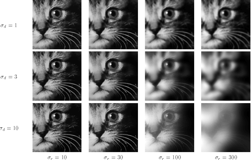
only whisker pixel values are averaged together. Figure 3 shows the effect of different values of the parameters
sigmad and sigmap on the resulting image. Rows correspond
to different amounts of domain filtering, columns to
different amounts of range filtering. When the value of the
range filtering constant sigma is large (100 or 300) with respect
to the overall range of values in the image (1 through 254),
the range component of the filter has little effect for small
sigmad: all pixel values in any given neighborhood have about
the same weight from range filtering, and the domain filter
acts as a standard Gaussian filter. This effect can be seen
in the last two columns of figure (3). For smaller values
of the range filter parameter sigma (10 or 30), range filtering
dominates perceptually because it preserves edges. However, for sigmad=10, image detail that was removed by
smaller values of sigmad reappears. This apparently paradoxical
effect can be noticed in the last row of figure 3, and in
particularly dramatic form for sigmar=100, sigmad=10. This
image is crisper than that above it, although somewhat hazy.
This is a consequence of the gray map transformation and
histogram compression results discussed in section 3. In
fact, sigmad=10 is a very broad Gaussian, and the bilateral
filter becomes essentially a range filter. Since intensity
values are simply remapped by a range filter, no loss of
detail occurs. Furthermore, since a range filter compresses
the image histogram, the output image appears to be hazy.
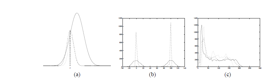
Figure 2 (c) shows the histograms for the input image and
for the two output images for sigmar=100, sigmad=3 and for
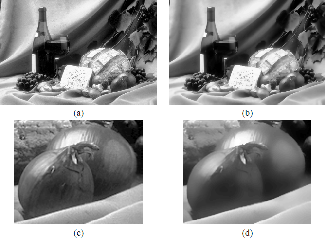
sigmar=100 , sigmad=10. The compression effect is obvious. Figure 4 (c) shows a detail of figure 4 (a), and figure
4 (d) shows the corresponding filtered version. The two
onions have assumed a graphics-like appearance, and the
fine texture has gone. However, the overall shading is
preserved, because it is well within the band of the domain Figure 2: (a) A unimodal image histogram v (solid)
, and the Gaussian similarity function s (dashed). (b) Histogram (solid)
of image intensities for the step in figure 1 (a) and (dashed) for the
filtered image in figure 1 (c). (c) Histogram of image intensities for the
image in figure 5 (a) (solid) and for the output images from figure 3. filter and is almost unaffected by the range filter. Also, the
boundaries of the onions are preserved. In terms of computational cost,the bilateral filter is twice
as expensive as a nonseparable domain filter of the same
size. The range component depends nonlinearly on the
image, and is nonseparable. A simple trick that decreases
computation cost considerably is to precompute all values
for the similarity function s(f). In the Gaussian case, if
the image has n levels, there are 2n+1 possible values for
S, one for each possible value of the difference fi-f. For black-and-white images, intensities between any
two grey levels are still grey levels. As a consequence,
when smoothing black-and-white images with a standard
low-pass filter, intermediate levels of gray are produced
across edges, thereby producing blurred images. With color
images, an additional complication arises from the fact that
between any two colors there are other, often rather different
colors. For instance, between blue and red there
are various shades of pink and purple. Thus, disturbing
color bands may be produced when smoothing across color
edges. The smoothed image does not just look blurred,
it also exhibits odd-looking, colored auras around objects.
Figure 6 (a) in the color plates shows a detail from a picture
with a red jacket against a blue sky. Even in this unblurred
picture, a thin pink-purple line is visible, and is caused
by a combination of lens blurring and pixel averaging. In
fact, pixels along the boundary, when projected back into
the scene, intersect both red jacket and blue sky, and the
resulting color is the pink average of red and blue. When
smoothing, this effect is emphasized, as the broad, blurred
pink-purple area in figure 6 (b) shows. To address this difficulty, edge-preserving smoothing
could be applied to the red, green, and blue components of
the image separately. However, the intensity profiles across
the edge in the three color bands are in general different.
Separate smoothing results in an even more pronounced pink-purple band than in the original, as shown in figure 6
(c). The pink-purple band, however, is not widened as it is
in the standard-blurred version of figure 6 (b). A much better result can be obtained with bilateral filtering.
In fact, a bilateral filter allows combining the three
color bands appropriately, and measuring photometric distances
between pixels in the combined space. Moreover,
this combined distance can be made to correspond closely
to perceived dissimilarity by using Euclidean distance in the
CIE-Lab color space [16]. This space is based on a large
body of psychophysical data concerning color-matching
experiments performed by human observers. In this space,
small Euclidean distances correlate strongly with the perception
of color discrepancy as experienced by an “average”
color-normal human observer. Thus, in a sense, bilateral
filtering performed in the CIE-Lab color space is the most
natural type of filtering for color images: only perceptually
similar colors are averaged together, and only perceptually
important edges are preserved. Figure 6 (d) shows the
image resulting from bilateral smoothing of the image in
figure 6 (a). The pink band has shrunk considerably, and
no extraneous colors appear. Figure 7 (c) in the color plates shows the result of five
iterations of bilateral filtering of the image in figure 7 (a).
While a single iteration produces a much cleaner image
(figure 7 (b)) than the original, and is probably sufficient
for most image processing needs, multiple iterations have
the effect of flattening the colors in an image considerably,
but without blurring edges. The resulting image has a much
smaller color map, and the effects of bilateral filtering are
easier to see when displayed on a printed page. Notice the
cartoon-like appearance of figure 7 (c). All shadows and
edges are preserved, but most of the shading is gone, and
no “new” colors are introduced by filtering. The literature on edge-preserving filtering is vast, and
we make no attempt to summarize it. An early survey can Figure 3: A detail fromg figure 5 (a)
processed with bilateral filters with range and domain parameter values Figure 4: A picture before (a) and after (b)
bilateral filtering. (c,d) are details from (a,b) be found in [8], quantitative comparisons in [2], and more
recent results in [1]. In the latter paper, the notion that
neighboring pixels should be averaged only when they are
similar enough to the central pixels is incorporated into
the definition of the so-called “G-neighbors.” Thus, Gneighbors
are in a sense an extreme case of our method, in
which a pixel is either counted or it is not. Neighbors in [1]
are strictly adjacent pixels, so iteration is necessary. A common technique for preserving edges during
smoothing is to compute the median in the filter’s support,
rather than the mean. Examples of this approach are
[6, 9], and an important variation [3] that uses K -means
instead of medians to achieve greater robustness. More related to our approach are weighting schemes
that essentially average values within a sliding window, but
change the weights according to local differential [4, 15]
or statistical [10, 7] measures. Of these, the most closely
related article is [10], which contains the idea of multiplying
a geometric and a photometric term in the filter kernel.
However, that paper uses rational functions of distance as
weights, with a consequent slow decay rate. This forces
application of the filter to only the immediate neighbors
of every pixel, and mandates multiple iterations of the filter.
In contrast, our bilateral filter uses Gaussians as a
way to enforce what Overton and Weimouth call “center
pixel dominance.” A single iteration drastically “cleans”
an image of noise and other small fluctuations, and preserves
edges even when a very wide Gaussian is used for
the domain component. Multiple iterations are still useful
in some circumstances, as illustrated in figure 7 (c), but
only when a cartoon-like image is desired as the output. In
addition, no metrics are proposed in [10] (or in any of the
other papers mentioned above) for color images, and no
analysis is given of the interaction between the range and
the domain components. Our discussions in sections 3 and
5 address both these issues in substantial detail. In this paper we have introduced the concept of bilateral
filtering for edge-preserving smoothing. The generality of
bilateral filtering is analogous to that of traditional filtering,
which we called domain filtering in this paper. The
explicit enforcement of a photometric distance in the range
component of a bilateral filter makes it possible to process
color images in a perceptually appropriate fashion.
The parameters used for bilateral filtering in our illustrative
examples were to some extent arbitrary. This is
however a consequence of the generality of this technique.
In fact, just as the parameters of domain filters depend on
image properties and on the intended result, so do those of
bilateral filters. Given a specific application, techniques for
the automatic design of filter profiles and parameter values
may be possible. Also, analogously to what happens for domain filtering,
similarity metrics different from Gaussian can be defined
for bilateral filtering as well. In addition, range filters can be
combined with different types of domain filters, including
oriented filters. Perhaps even a new scale space can be
defined in which the range filter parameter sigmar corresponds
to scale. In such a space, detail is lost for increasing sigmar, but
edges are preserved at all range scales that are below the
maximum image intensity value. Although bilateral filters
are harder to analyze than domain filters, because of their
nonlinear nature, we hope that other researchers will find
them as intriguing as they are to us, and will contribute to
their understanding. 1. T. Boult, R. A. Melter, F. Skorina, and I. Stojmenovic. G-neighbors.Proc. SPIE Conf. on Vision Geometry II, 96–109, 1993.Experiments with Black-and-White Images
Experiments with Color Images
Relations with Previous Work
Conclusions
References
2. R. T. Chin and C. L. Yeh. Quantitative evaluation of some edgepreserving
noise-smoothing techniques. CVGIP, 23:67–91, 1983.
3. L. S. Davis and A. Rosenfeld. Noise cleaning by iterated local
averaging. IEEE Trans., SMC-8:705–710, 1978.
4. R. E. Graham. Snow-removal—a noise-stripping process for picture
signals. IRE Trans., IT-8:129–144, 1961.
5. N. Himayat and S.A. Kassam. Approximate performance analysis
of edge preserving filters. IEEE Trans., SP-41(9):2764–77, 1993.
6. T. S. Huang, G. J. Yang, and G. Y. Tang. A fast two-dimensional
median filtering algorithm. IEEE Trans., ASSP-27(1):13–18, 1979.
7. J. S. Lee. Digital image enhancement and noise filtering by use of
local statistics. IEEE Trans., PAMI-2(2):165–168, 1980.
8. M. Nagao and T. Matsuyama. Edge preserving smoothing. CGIP,
9:394–407, 1979.
9. P. M. Narendra. Aseparable median filter for image noise smoothing.
IEEE Trans., PAMI-3(1):20–29, 1981.
10. K. J. Overton and T. E. Weymouth. A noise reducing preprocessing
algorithm. In Proc. IEEE Computer Science Conf. on Pattern
Recognition and Image Processing, 498–507, 1979.
11. Athanasios Papoulis. Probability, random variables, and stochastic
processes. McGraw-Hill, New York, 1991.
12. P. Perona and J. Malik. Scale-space and edge detection using
anisotropic diffusion. IEEE Trans., PAMI-12(7):629–639, 1990.
13. G. Ramponi. A rational edge-preserving smoother. In Proc. Int’l
Conf. on Image Processing, 1:151–154, 1995.
14. G. Sapiro and D. L. Ringach. Anisotropic diffusion of color images.
In Proc. SPIE, 2657:471–382, 1996.
15. D. C. C. Wang, A. H. Vagnucci, and C. C. Li. A gradient inverse
weighted smoothing scheme and the evaluation of its performance.
CVGIP, 15:167–181, 1981.
16. G. Wyszecki andW. S. Styles. Color Science: Concepts and Methods,
Quantitative Data and Formulae. Wiley, New York, NY, 1982.
17. L. Yin, R. Yang, M. Gabbouj, and Y. Neuvo. Weighted median
filters: a tutorial. IEEE Trans., CAS-II-43(3):155–192, 1996.