
In this paper, we propose a mathematical model and an adaptive large neighborhood search to solve a two{tiered transportation problem arising in the distribution of goods in congested city cores. In the first tier, goods are transported in city buses from a consolidation and distribution center to a set of bus stops. The main idea is to use the buses spare capacity to drive the goods in the city core. In the second tier, final customers are distributed by a eet of near-zero emissions city freighters. This system requires transferring the goods from buses to city freighters at the bus stops. We model the corresponding optimization problem as a variant of the pickup and delivery problem with transfers and solve it with an adaptive large neighborhood search. To evaluate its results, lower bounds are calculated with a column generation approach. The algorithm is assessed on data sets derived from a _eld study in the medium-sized city of La Rochelle in France.
Keywords: City logistics, Pickup and Delivery Problem with Transfers, Adaptive Large Neighborhood Search, mixed passengers and goods transportation.
1 Introduction
Urban mobility significantly contributes to achieving socioeconomic objectives of cities but at the same time it impacts on city living conditions in terms of congestion, emission and pollution. Nowadays, cities are looking for instruments and policies to ensure an efficient and effective urban mobility for both passengers and goods. For this purpose, it is essential to manage urban mobility considering passengers and goods flows as a single logistics system (European Commission, Directorate-General for Energy and Transport, 2007). This flows streamlining can be obtained through consolidation and coordination. That means less vehicles traveling within the city and a better use of these vehicles. Different city logistics systems have been proposed and implemented in several cities, including cooperative freight transport systems and advanced information systems. However, only few systems considered the passengers and goods flows together.
In this paper, we investigate the management of urban transportation flows making a joint use of transport resources between passengers and goods. The main idea is to use the spare capacity of city buses to carry goods into the city core. This idea has emerged in the context of B2B parcel delivery by near zero emissions vehicles. These vehicles, called city freighters can be electrically-assisted tricycles, electric cars, etc. Contrary to trucks, city freighters have low impact on congestion and can park easily. The counterpart is their limited capacity, which forces them to be replenished several times a day. Hence, delivering with small capacity vehicles is profitable only if vehicles are loaded close enough to their customers. This motivates the use of public transportation to bring the parcels to the last kilometer.
In practice, we study a logistics network composed of a warehouse called CDC (Consolidation and Distribution Center), a bus line and a set of customers. We assume that the CDC is easily accessible by truck and connected to the bus line. All goods proceeding from the city outdoors are collected and stored at the CDC before being delivered.
The goal of this paper is to compare two distribution systems. In the conventional approach, parcels are delivered from the CDC to the customers with a fleet of homogeneous electric trucks. This amount to solve instances of the well-known vehicle routing problem with time windows (VRPTW). This is depicted in Figure 1.
The second approach is a two-tiered transport system. In the first tier, goods are carried by city buses from the distribution center to a number of bus stops in the city core. In the second tier, goods are delivered to final customers by a fleet of city freighters. This approach is represented in Figure 2.

The concept of two{tiered city logistics system mixing passengers and goods has been proposed in Trentini and Malhene (2010) and Trentini et al. (2011). The main contribution of this paper is to propose a quantitative assessment for such a system. First, we propose a mathematical model to minimize the number of vehicles allowing the satisfaction of the daily customer demands. Then, we solve this model with a meta-heuristic called Adaptive Large Neighborhood Search (ALNS).
The remaining of this paper is organized as follows. Section 2 presents the optimization problem, proposes a mathematical formulation and positions it in the operational research literature. Section 3 describes the ALNS algorithm used to solve the optimization problem. In section 4, we focus on a sub-problem concerning the feasibility of inserting a customer in a partial solution. Section 5 presents a column generation approach to calculate good lower bounds of the number of city freighters required. Finally, in section 6 we detail the computational experiments led on a case study in the city of La Rochelle (France).
2 The Mixed Urban Transportation Problem
In this section, we _rst provide a description of the problem, introduce some notations and formulate the optimization problem as a Mixed Integer Program (MIP) before presenting and discussing the related literature.
2.1 Problem description
The Mixed Urban Transportation Problem (MUTP) consists in delivering parcels to shops and administrations – called customers – located in the city center. These customers have frequent demands (daily or several times a week), but the demanded quantities and the customers locations vary from one day to another. Since the problem is solved everyday with new demands, we consider a scheduling horizon of one day. In addition, our problem includes a single bus line, with a known schedule. Without loss of generality, we assume that the bus line starts at the CDC.
Operations at the CDC The CDC is in charge of three operations:
reception: collecting parcels coming from outside the city;
sorting: loading parcels into a set of rolling containers such that one customer demand is placed into a single container;
shipping: loading rolling containers onto buses, such that their spare capacity is respected.
We assume that the demand is known at the beginning of the day and that the system is asynchronous: all reception and sorting operations are terminated before shipping begins. In our case study, the logistics operations are performed once a day. The proposed approach also applies when multiple campaigns are performed everyday.
Loading buses
The schedule of each bus is known and the occupancy rate at each station has been estimated in a preliminary field study. From this data, we deduced the maximal number of containers that can be loaded into each bus without deteriorating the quality of service delivered to passengers. Another important factor impacting the quality of service is the duration of loading and unloading operations at bus stops. In order to limit this duration, adequate container systems and bus access have to be used (Trentini and Malhene, 2010). Moreover, we impose a maximal number of containers that can be loaded or unloaded simultaneously at a given station.
Transshipment from buses to city freighters
The rolling containers are carried by buses from the CDC to some bus stops, where they are unloaded and transshipped to city freighters. As the number of containers allowed in a bus is small, we assume that unloading operations take a constant time. The content of the containers is not modified during the transshipment. In order to minimize the system cost, we assume no storage facility at bus stops. This involves synchronizing buses and city freighters: each time a container is unloaded from a bus, there must be a city freighter waiting for it there. We consider a fixed time for the operation consisting of unloading the roll containers from the bus and loading them on city freighters.
Last kilometer
The last kilometer is operated by city freighters. Each city freighter starts and finishes its working day at some depot and visits a sequence of customers. Each customer has a delivery time window. If a city freighter arrives at a customer before the opening of the time windows, it has to wait. Late arrivals are not allowed. We define trips and routes as follows.
De_nition 2.1 A trip is an itinerary performed by a city freighter, starting at a bus stop and visiting a sequence of customers.
In this study, we consider only trips for which (i) the whole demand of a customer is served by a single trip, (ii) a trip delivers the whole content of a rolling container.
A trip it said to be feasible if each customer in the trip is visited once, within its time window.
Denition 2.2 A route is the complete itinerary of a city freighter in the scheduling horizon. A route consists of an initial depot, followed by a sequence of trips, and a final depot.
Note that a city freighter can visit several bus stops within a route in order to better fit the demand. In Figure 2, this is the case of city freighter 2.
Objective
The goal of the mixed transportation system is to reduce the global impact of deliveries in the city, including various factors such as cost, CO2 emissions, traffic congestion, noise, infrastructure, inconvenience caused by parked vehicles, etc. Designing a mixed passengers and goods transportation system is a multidisciplinary project by nature (Trentini and Malhene, 2010). The objective of this paper is to assess the feasibility and logistic efficiency of such a system. Thus, our main criteria is the impact of the new system on the existing infrastructure. As a result, we focus on the number of city freighters required to satisfy the customer demands, and their utilization (distance traveled, occupation of bus stops etc.).
2.2 Notations
We consider a set N of customers. Each customer i ϵ N has a demand qi that must be delivered during its time window [ei; li]. This demand is assumed to be less than or equal to the capacity of one roll and not splittable among several containers.
The bus set is denoted by B. We consider that each bus departure from the CDC corresponds to a bus b with a residual capacity of Qb containers. The set S represents the bus stops. It consists of the CDC and all stops where containers can be unloaded from buses. At each bus stop s ϵ S, at most Qs containers can be loaded or unloaded simultaneously.
The set T = B x S models the service of all stops in S by each bus in B. For each i ϵ T, we denote by hi the service time of i provided by the bus schedule. The subset Ts ⊂ T represents the visits of all buses to bus stop s ϵ S. The subset Tb ⊂ T represents the visits of bus b ϵ B to all bus stops. The second tier is operated by a homogeneous feet K of city freighters having a capacity of one roll. Each city freighter has its own initial and final depot. The sets of initial and ending depots are denoted by O and O’, respectively. In practice, O and O’ can represent a single physical location.
The optimization problem modeled in the next section is defined on a graph G = (V; A). The set V of vertices includes all customers, depots and bus visits: V = N ∪ O ∪ O’ ∪ T. Each vertex i ϵ V is associated with a service duration σi representing either the time to load/unload a container or the time to serve a customer. For all o ϵ O ∪ O’, we consider that σo = 0. The set A of arcs contains all arcs that can be used in a solution. A ∪ (O x T) ∪ (T x N) ∪ (N x N) ∪ (N x T) ∪ (T x T) ∪ (N x O’) ∪ (O x O’). Each arc (i; j) ϵ A is associated with a known travel time ti;j and a cost ci;j.
Some arcs can be discarded due to temporal constraints. For example there exist no arc (i; j); i ϵ T; j ϵ T such that hi + ti;j > hj . Note that arcs between an initial and an ending depot are taken by city freighters which are not utilized.
The definition of a trip can now be formally expressed on graph G.
Proposition 2.1 A trip on graph G = (V;A) is an elementary path on G that is composed of one vertex i ϵ T, followed by a sequence of customers in N.
In this model, the two tiers in the transportation system are linked through vertices in T.
2.3 Mathematical formulation
We now introduce a mathematical model of the MUTP. For each arc (i; j) ϵ A, we define a decision variable xi;j ϵ {0; 1} that is equal to 1 if a city freighter uses (i; j), and 0 otherwise. For all i ϵ N, variables ui ϵ [0; 1] model the filling rate of the city freighter that serves i when it leaves this vertex. For all i ϵ V , the value hi ϵ [ei; li] denotes the time of service at customer i. An important remark is that hi is a variable if i ϵ N ∪ O ∪ O’ and a known bus time, given in the schedule, if i ϵ T.
We use a classical approach in vehicle routing, which consists in lexicographically minimizing two objective functions. The first objective is the number of city freighters necessary to serve every customer. The second objective is the sum of arc costs.
According to the previously introduced notation, the MUTP can be modeled as follows:

Constraints (2) and (3) state that each city freighter starts from its initial depot and returns to its ending depot. Constraints (4) ensure that each customer is served by exactly one vehicle. Constraints (5) are flow conservation constraints. Constraints (6) update load variables that enforce the satisfaction of container capacity. Note that this constraint is not set when j is a bus stop, which allows the city freighters to be replenished at this vertex. Constraints (7) establish the relationship between a vehicle service time from a vertex and its immediate successor. This also models the synchronization constraints at bus stops where service times are fixed. Note that city freighters that visit the same bus stop are served simultaneously. Constraints (8) limit the number of containers that can be unloaded simultaneously at a transshipment point. Constraints (9) ensure that the capacity of buses is respected. Finally constraints (10)-(12) define the domains of the variables. Constraints (6) and (7) can be linearized using classical big M techniques (Cordeau et al., 2002), but this makes the solution of this model by an MILP solver very inefficient.
2.4 Position in the OR literature
The MUTP falls into the large family of vehicle routing problems, and more particularly two-tiered problems. Solving the single-tiered city logistics system amounts to solving a very classical problem in the field of operations research: the Vehicle Routing Problem with Time Windows (VRPTW). For more details, one can refer to Cordeau et al. (2002). Single-tiered city logistics systems where consolidation activities take place at CDC are frequent and are generally sufficient for medium-sized cities. Long-haul transportation vehicles dock at a CDC to unload their goods. Loads are then sorted and consolidated into smaller vehicles for distribution (Crainic et al., 2009). Single{tiered systems suppose that those vehicles can be parked easily in the customer area, which is not the case in our study.
Two-tiered or multi{tiered systems have been emerging in the last ten years in the field of city logistics. Crainic et al. (2009) consider a system where the first tier consolidates loads at CDC into vehicles, which bring them to smaller facilities called satellites, close to or in the city center. The second tier uses smaller vehicles called city freighters to deliver the goods to the customers. A particular case of the underlying optimization problem is the Two-Echelon Vehicle Routing Problem (2E-VRP).
The MUTP shares some similarities with the 2E-VRP and with the Pickup and Delivery Problem with Transfers (PDPT). In order to position the MUTP, we present a non-exhaustive literature review of these two problems.
The Two-Echelon Vehicle Routing Problem and related problems
Perboli et al. (2011) introduce multi-tiered vehicle routing problems, and focus on the two-tiered case. The authors present several versions of 2E-VRP considering synchronization of vehicles at satellites or time windows. Synchronization at satellites requires the presence of both the first and the second echelon vehicles at a satellite when a load is transferred. In the case with no synchronization nor time window, the authors introduce a mathematical model solved with an MILP solver. To solve larger instances, two matheuristics based on the mathematical model are proposed. These matheuristics and the MILP results are compared on instances considering up to 50 customers and 4 satellites.
This recent study has been followed by numerous works to solve the 2E-VRP. Perboli and Tadei (2010) present several families of valid inequalities for the model of Perboli et al. (2011). They show that adding these inequalities enables solving larger instances to optimality. Crainic et al. (2011) introduce a two-stage heuristic method that outperforms the matheuristics of Perboli et al. (2011). Hemmelmayr et al. (2012) introduce an ALNS with eight destroy and five repair operators. The authors evaluate the method on a set of 93 instances (Crainic et al., 2010; Perboli et al., 2011) for which 59 new best solutions are identified. In addition, a branch-and-cut method has been designed by Jepsen et al. (2012) and a branch-and-price approach by Roberti (2012).
A configuration analysis is proposed in Crainic et al. (2010) regarding the position of the depot, the number of requests and their spatial repartition. The benefits of the multi-tiered approach appears to be higher when the CDC is located outside the customers area. This is generally the case in city logistics: CDC are usually located at the edge of the city.
Note that the 2E-VRP supposes one trip per vehicle in all approaches. A related problem which integrates multiple trips but no load transfer has been introduced by Crainic et al. (2012b). They focus on designing the routes from satellites spread in multiple zones to customers. The time of a satellite delivery is known. A vehicle that starts from a satellite should be present when goods are delivered. In Crainic et al. (2012b), a two stages solution method and lower bounds are proposed to solve instances with up to 3600 customers. On this problem, Nguyen et al. (2013) propose a tabu search and provide significant improvements to the previous results. Also related, Cattaruzza et al. (2013) introduce the Multi-Trip Vehicle Routing Problem with Time Windows and Release Dates where goods are distributed by small vehicles performing multiple trips from a single CDC. Goods are delivered all over the day at the CDC by semi-trailers. The time at which a set of goods is made available for distribution is called a release date. The problem is solved with a memetic algorithm.
The Pickup and Delivery Problem with Transfers
Compared to the well known Pickup and Delivery Problem (PDP), the PDPT relaxes the constraint that requests are carried from their pickup point to their delivery point by the same vehicle. The requests may be transferred from one vehicle to another at some predetermined locations.
The first work considering the opportunity of transferring requests in a PDP context is due to Stein (1978). In this work neither the capacity of vehicles nor the time windows on points are taken into account. Shang and Cuff (1996) present a heuristic for a PDPT where every vertex can be used as a transfer point. Transfer is considered as a recourse when inserting a request in the current solution would imply the use of an additional vehicle. Cortes and Jayakrishnan (2002) develop a simulation for a demand-responsive transit system that allows a single transfer per passenger. Mitrovic-Minic and Laporte (2006) present a local search for a PDPT with uncapacitated vehicles. They present extensive experiments with up to 100 requests. Grtz et al. (2009) propose heuristics for a PDPT with capacitated and uncapacitated vehicles, with the objective of minimizing the makespan. Petersen and Ropke (2011) present an LNS for a PDP with a single transfer point. The algorithm is applied to the distribution of flowers in Denmark, the instances contain up to 982 requests. Qu and Bard (2012) propose a GRASP coupled with an ALNS and evaluate it on instances with up to 25 requests. Masson et al. (2012a) develop an ALNS and present competitive results on the instances of Mitrovic-Minic and Laporte (2006). A focus on request insertion feasibility algorithms is given in Masson et al. (2013a). These algorithms are extended to tackle the dial a ride problem with transfers (Masson et al., 2012c,b).
Few exact approaches have been designed to solve the PDPT. Cortes et al. (2010) first proposed a mathematical formulation of the PDPT and solved instances with up to six requests using a branch-and-cut algorithm. Kerivin et al. (2008) present a mathematical formulation for a version of the problem without any time windows. Instances with up to 15 requests are solved using a branch-and-cut algorithm. Fugenschuh (2009) solve a school bus problem where routes are already designed and need to be assigned to a minimum number of vehicles. Some passengers can be transferred from one bus to another. Masson et al. (2013b) present a branch-and-cut-and-price for a special case of the PDPT with only a few delivery locations and where a vehicle is not allowed to visit more than two distinct delivery locations. Instances with up to 87 customers are solved to optimality in less than 1 hour.
3 An Adaptive Large Neighborhood Search for the Mixed Urban Transportation Problem
The two criteria minimized in a lexicographical way in the MUTP are the number of city freighters used and the total distance traveled. Therefore, the assignment of containers to buses does not influence the cost of the solution. For a given set of city freighters routes in the second tier, the problem in the first tier only consists in finding a feasible assignment of containers to buses.
Thus, we propose to decompose the MUTP into a master problem and a sub-problem. The master problem consists in designing the city freighters routes, which answers the following questions:
How are the parcels dispatched into containers?
At which bus stop a container is unloaded from a bus to a city freighter?
Which container is assigned to which city freighter?
What is the optimal sequence of customers in a trip?
How to sequence the trips of city freighters?
The sub-problem consists in finding a feasible assignment of containers to buses. For each stop s ϵ S and each container unloaded at s, we determine which vertex i ϵ Ts links the two tiers of the transportation system. Since the assignement of containers to buses has no impact on the objective function, the sub-problem is only a feasibility problem: we look for an assignment that satisfies bus capacity constraints and customers time windows.
The master problem is solved with an ALNS, described in section 3.1. The sub-problem presented in section 4 is solved within the ALNS, each time a customer insertion is evaluated.
3.1 Adaptive Large Neighborhood Search
Large Neighborhood Search (LNS) has been introduced by Shaw (1998) in a constraint programming framework to solve the VRPTW. LNS is similar to the ruin and recreate method introduced by Schrimpf et al. (2000). Pisinger and Ropke (2010) present an extensive survey of the method and its application to combinatorial optimization problems. As depicted in Algorithm 1, the underlying principle of the LNS is to iteratively partially destroy and repair a solution in order to improve it.
Algorithm 1 LNS
Require: An initial solution S0
1: BestSolution ←S0
2: CurrentSolution ← S0
3: while the termination criterion is not satisfied do
4: Selection of Destroy and Repair heuristics
5: S ← CurrentSolution
6: S ← Destroy(S)
7: S ← Repair(S)
8: if S < BestSolution then
9: BestSolution ← S
10: CurrentSolution ← S
11: else
12: if NewSolutionAccepted(S) then
13: CurrentSolution ← S
14: return BestSolution
LNS relies on repetitive use of problem dependent heuristics for destroying and repairing the current solution (lines 4-7). The resulting solution is saved when it dominates the preceding ones (lines 8-10) and it may be accepted even if it deteriorates the objective function during the search (line 11-13). In this case, the most common acceptance criteria come either from Simulated Annealing (Kirkpatrick et al., 1983) or from the Record-to-Record Travel algorithm (Dueck, 1993).
Adaptive Large Neighborhood Search (ALNS) (Ropke and Pisinger, 2006a) is an extension of LNS which adaptively combines the destroy and repair operators. The search is called adaptive because the probability of choosing each operator depends on its efficiency during the previous iterations. ALNS has been proven very efficient to solve a large range of Vehicle Routing Problems (Pisinger and Ropke, 2007a; Ropke and Pisinger, 2006b). In particular, this method has been applied with success to solve both the 2E-VRP (Hemmelmayr et al., 2012) and the PDPT (Masson et al., 2012a). Since ALNS is now widely used for solving vehicle routing problems, we focus on the destroy and repair operators that have been designed to solve the MUTP and refer to Ropke and Pisinger (2006a) for a complete description of the ALNS algorithmic framework.
3.2 Destroy operators
We have implemented four distinct destroy operators, either adapted from Ropke and Pisinger (2006b) or Masson et al. (2012a).
Random removal: this heuristic randomly selects p% of the customers to be removed from the current solution.
Worst removal: this heuristic first computes the detour caused by each customer in the city freighter trip. p% of the customers are then selected randomly for removal. The probability of being selected increases with the value of the detour. Transfer point removal: this heuristic randomly selects one bus stop s ϵ S and destroys all trips originating from this stop.
Related removal: this heuristic aims at removing related entities in a solution. The relatedness measure is problem dependent. We define the relatedness measure between two customers i ϵ N and i’ ϵ N as the value

First, a seed request is selected randomly. Then the relatedness between the seed request and each planned request is computed. Based on this measure, a request is removed with a probability that increases when its relatedness measure decreases.
3.3 Repair operators
Two distinct repair operators are used in the LNS.
Best insertion: for each customer, its best insertion position in each city freighter route is evaluated. The customer with the cheapest insertion cost is inserted at its best position. This operation is repeated until no more customer can be inserted.
For a given customer, the search for its best insertion position is described in Algorithm 2. This algorithm first evaluates the insertion of customer c ϵ N in a new trip at the beginning of the route (lines 1-2). Then, the best insertion position is sought among every possible position in the existing trips of the route (lines 3-5). In addition, the insertion of c in a new trip is tested after all existing trips (lines 6-7).
This algorithm is illustrated in Figures 3 and 4. Let S = {s1; s2}. Figure 3 represents a city freighter route, composed of two trips denoted by τ1 = (s1 → c1 → c2) and τ2 = (s2 → c3).

Figure 4 lists all routes evaluated by Algorithm 2 on this example. Evaluating an insertion position consists of checking its feasibility and evaluating the resulting cost increase. The feasibility checking algorithm is described in Section 4.
Algorithm 2 Best insertion of a customer in a city freighter route
Require: a customer c ϵ N; a city freighter route r.
1: for all s ϵ S do
2: evaluate the insertion of a trip (s → c) after the initial depot of r
3: for every trip τ in r do
4: for every vertex i ϵ τ do
5: evaluate the insertion of c after node i
6: for all s ϵ S do
7: evaluate the insertion of a new trip (s → c) after trip τ
8: return the best feasible position of insertion

Most constrained first: this repair operator is a variant of the best insertion procedure. At each iteration, in order to favor feasibility, the customer that can be inserted in the smallest number of trips is inserted first. Cost is used as a second selection criterion for tie breaking.
3.4 Minimizing the number of required vehicles
The first objective function of the MUTP is to minimize the number of city freighters used to serve all customers. We follow a two-stage approach proposed by Ropke and Pisinger (2006a), in which the first stage aims at minimizing the number of vehicles used. In this first stage, an initial solution that serves all customers is first built. It determines an initial number of routes. Next, one route is removed from the solution and its customers are placed in a request bank. The resulting problem is solved by the ALNS with an objective function that minimizes a weighted sum of two terms: the sum of arc costs and the number of requests in the request bank, which is penalized with a very high weight. Everytime a solution that serves all customers is found, one route is removed and the process is repeated until a fixed number of ALNS iterations is reached. The number of vehicles in the solution is then determined by the best solution with all requests served.
4 Checking the feasibility of an insertion Let us consider a partial solution resulting from the destroy operations
Let us consider a partial solution resulting from the destroy operations in the ALNS. The repair operations in the ALNS sequentially insert customers into feasible partial routes. Each insertion requires checking whether buses capacities, stops capacities and time windows constraints are still satisfied. We call this feasibility problem the Rolling Containers Assignment Problem (RCAP). This problem amounts to determine the starting vertex in t ϵ Ts of each trip.
The trips are performed sequentially. Therefore, there is a precedence constraint between trips. In the example of Figure 3, trips τ1 and τ2 must be assigned to two buses such that the city freighter arrives at s2 before time hs2, i.e. before the arrival of the bus carrying the container of trip τ2.
The RCAP consists in assigning each rolling container to a bus such that (i) the bus capacity is respected, (ii) the maximal number of containers transferred simultaneously at a bus stop is respected, (iii) the customer time windows are satisfied, (iv) the synchronization constraints between bus and city freighters at bus stops are satisfied.
In section 4.1, we propose a mathematical model for the RCAP. A sufficient condition to accept a customer insertion in a route is then proposed in section 4.2. This condition is incorporated into the ALNS algorithm.
Note that checking that the capacity of a container is not exceeded is done in repair operators
before solving the RCAP.
4.1 Mathematical model of the Rolling Containers Assignment Problem
Let T be the set of trips in all city freighters routes. For all τ ϵ T, we denote by τ+ the successor of trip τ, or the ending depot if τ is the last trip. We also denote by s(τ) ϵ S the starting stop of trip τ. For each s ϵ S, the set of trips beginning at bus stop s is written Ts.
The model is based on the definition of three values for each trip τ ϵ T : The minimal trip duration of trip represents its duration when the city freighter never waits for the opening of the time window at a customer. The earliest finishing time of trip τ is the earliest possible arrival time at the starting bus stop s(τ+) of τ+. The latest starting time of trip τ is the latest time at which trip τ can start without violating any time window constraint.
Definition 4.1 Let τ ϵ T be a trip that sequentially visits locations v0,…, vn, where v0 = s(τ),v1,…, vn ϵ V denote its customers and vn+1 = s(τ+). Let us denote by tv0;v1 and tvn;vn+1, the travel times from v0 to v1 and from vn to vn+1, respectively. σv0 denotes the service duration at stop v0. Then:

According to these notations we can formulate the following proposition which is a reformulation of the Forward Time Slack principle of Savelsbergh (1992):
Proposition 4.1 Let wτ and wτ+ be the starting time of trip τ and τ+, respectively. The time windows of the customers served by are satisfied if and only if wτ ≤ $\overline{l}$τ and max(wτ+mτ; $\overline{e}$τ ) ≤ wτ+.
The RCAP model uses variables wτ introduced in Proposition 4.1 and for each trip τ ϵ T and each bus b ϵ B, the binary variables zτ;b, which are equal to 1 if the container of trip τ is unloaded from bus b and 0 otherwise. In addition, we denote by hbs the known service time of a stop s ϵ S by a bus b ϵ B.
The RCAP is feasible if and only if variables zτ;b and wτ can be given values such that:
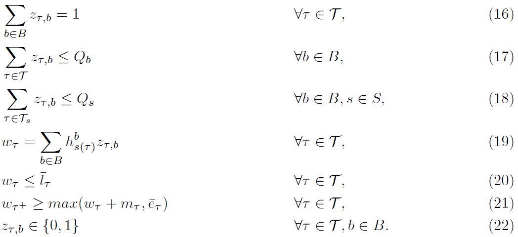
Constraints (16) guarantee that each trip is assigned to exactly one bus. Constraints (17) guarantee that buses capacities are respected. Similarly, constraints (18) ensure that bus stops capacities are respected. Constraints (19) set the starting time of each trip to the time at which its assigned bus visits s(τ). Constraints (20) and (21) result from Proposition 4.1 and prevent time windows violations. Finally, constraints (22) define the domain of variables zτ;b.
4.2 A heuristic for checking the feasibility of an insertion
To the best of our knowledge, there is no polynomial time algorithm to solve the RCAP. As this problem is solved to validate numerous insertions in repair operators of the ALNS, it requires a very fast solution method. Thus, we propose a heuristic test based on a sufficient condition for the feasibility of a customer insertion in a partial solution.
Let us consider the insertion of a customer i in a route r and let us suppose that the schedules and assignments of other routes are left unchanged. Verifying the city-freighter capacity constraint for route r is straightforward. We focus on checking the feasibility of a customer insertion in r with respect to time windows, buses and stops capacities. For each vertex j ϵ r, we define the $\overline{l}$j value, which is the latest starting time of the trip at j, given the current schedules and assignments of the other routes. Note that for each trip τ ϵ r, if j is the first vertex of τ then $\overline{l}$j is a lower approximation of $\overline{l}$τ . If, for each j ϵ r, a service time wj can be found such that wj ≤ $\overline{l}$j , then a feasible schedule exists.
Algorithm 3 computes the $\overline{l}$j values from the last vertex to the first of a route r.
Algorithm 3 Heuristic calculation of latest service times ~lj for each vertex j in route r
Require: A city freighter route r with final depot o’
1: j’ ← o’, $\overline{l}$j’ ← lo’ {j’ designs the successor of vertex j in r}
2: for each trip τ ϵ r, from last to first do
3: for each vertex j ϵ τ , from last to first do
4: $\overline{l}$j ← min(lj ; $\overline{l}$j’ – σj’ – tj;j’)
5: j’ ← j
6: Let b* ϵ B be the latest bus in the solution that can serve trip τ through stop j = s(τ ).
7: $\overline{l}$j ← hs(τ )b*
Note that, when executing line 6, vertex j is the starting bus stop of trip τ to which a bus b* should be assigned, taking account of: the already assigned trips in this route, the trip assignments in other routes, and provided that:
the capacity of the bus Qb is not exceeded,
the capacity of the bus stop Qs(τ ) is respected for this bus,
hs(τ ) b* is less than or equal to the latest service time $\overline{l}$j computed in the previous loop.
Considering that each vertex j in route r is served at time wj in an “as early as possible” schedule, the sufficient condition for the feasibility of the insertion of a vertex i between two vertices j and j’ is expressed as follows:
Proposition 4.2 Let us consider a trip τ ϵ T and two consecutive vertices j and j’ in τ. The insertion of a vertex i between j and j’ in trip τ is feasible if

Two cases are considered when a customer is inserted in a solution: either the customer is inserted in an existing trip, or a new trip is created (see Algorithm 2). Each time the ALNS evaluates the insertion of a customer in a partial solution of the MUTP, the two types of insertions are treated as follows:
Insertion in an existing trip: according to Proposition 4.2 we compute the earliest possible service time for the customer to be inserted, and check that the successor vertex can be visited before its latest possible service time. This test can be performed in constant time.
Insertion in a new trip: we determine the first bus capable of servicing the new trip, and proceed like in the preceding case. This test can then be performed in a time that is linear with the number of buses.
In conclusion, all temporal constraints related to the insertion of a customer in a trip can be reduced to constraints on its starting time w . However, solving the exact feasibility problem remains hard. Proposition 4.2 gives a sufficient feasibility condition that can be checked very efficiently. If an insertion does not satisfy the sufficient condition, the repair operator of the ALNS considers it as unfeasible.
5 A lower bound for the number of used city-freighters
The ALNS introduced in section 3 provides upper bounds of the MUTP optimal solutions. In order to compute lower bounds and evaluate the results obtained with the ALNS, we propose a set-partitioning formulation for the MUTP, with the single objective of minimizing the number of vehicles. The linear relaxation of this formulation is solved by column generation.
5.1 A set-partitioning formulation for route minimization in the MUTP
Let us denote by Ω the set of all possible routes. A route r ϵ Ω is characterized by a vector ar where: ajr takes value 1 if route r visits vertex j ϵ N, and ar(b;s) = 1 if r visits the stop s of bus b. For all r ϵ Ω we introduce a binary variable yr that takes value 1 if and only if route r is used in the solution of the problem.
According to this notation, the set-partitioning formulation of the MUTP can be given as follows:

The objective function (23) minimizes the number of city freighters used. Constraints (24) state that each customer must be visited exactly once. Constraints (25) ensure that buses capacities are respected. Constraints (26) ensure that bus stops capacities are respected.
5.2 Solving the linear relaxation of the set-partitioning formulation
Set-partitioning formulations of vehicle routing problems generally includes millions or billions of decision variables. It is therefore not possible to explicitly enumerate all these variables. The general idea of column generation is to solve a linear relaxation which only considers a small subset of decision variables. If the result of this restricted problem is optimal, the algorithm stops. Otherwise, columns that correspond to negative reduced cost variables are generated. This amount to solve a sub-problem called a pricing problem. If such columns are identified, they are appended to the restricted set of columns and the problem is solved again. This process is repeated as long as the sub-problem admits columns with a negative reduced cost. Column generation provides tight lower bounds for vehicle routing and has been successfully applied to solve the related Pickup and Delivery Problem with Time Windows (Ropke and Cordeau, 2009), (Baldacci et al., 2011) or the Pickup and Delivery Problem with Shuttle Routes (Masson et al., 2013b). For a didactic and complete description of the implementation of column generation in vehicle routing, we refer to Feillet (2010).
In this paper, we solve the linear relaxation of (23) – (27) by column generation. The two key elements to implement this lower bound are the calculation of the reduced cost and the identification of the sub-problem.
Let πi be the dual variables associated with constraints (24), π’b the dual variables associated with constraints (25) and π’’b,s the dual variables associated with constraints (26).
The reduced cost of a variable yr; r ϵ Ω is:

Finding a column with a negative reduced cost is equivalent to finding an elementary shortest path that represents a feasible route on graph G where: an arc in A that leaves a customer i ϵ N takes’ cost πi, an arc that leaves a vertex that represents the stop of a bus b ϵ B at s ϵ S takes cost π’b + π’’b,s, other arcs have cost 0.
This sub-problem can be modeled as an Elementary Shortest Path Problem with Resource Constraints (ESPPRC). The considered resources are the capacity of a vehicle and the time. We use the algorithm proposed by Feillet et al. (2004) to solve this problem.
6 Computational experiments
Section 6.1 evaluates the reliability of the ALNS by comparing its results with the lower bound on small instances. The case study that motivated this paper is then introduced in section 6.2. We compare the conventional distribution approach with large vehicles (Figure 1) to the mixed urban transportation system (Figure 2). The experiments are run on a set of instances built from real-life data.
6.1 Comparison with lower bounds
In order to validate the efficiency of the proposed ALNS method, we first compare the number of vehicles obtained by this method with the lower bound obtained by the column generation approach. As this is the primary objective of the study, we focus on minimizing the number of vehicles.
To this end, we generated a set of instances with 50 customers, 5 buses and 5 bus stops. The instances are divided into three categories in which the geographical distribution of vertices is random (R), clustered (C) or mixed random/clustered (RC). We also consider two service durations: in instances of type A, customers have a service duration of 5 minutes whereas it is 10 minutes in instances of type B.
The ALNS algorithm is run 5 times for 2 minutes on each instance, its results are reported in Table 1. The instance names in the first column are of the form X-Y-Z where X ϵ {R,C,RC} is the type of geographical distribution, Y ϵ {A,B} is the type of service duration and Z ϵ {1,2,3} is an instance number. The second column reports the lower bound LB(z) obtained by the column generation approach. The third and fourth columns report the best result (min(z)) and the average result (avg(z)) obtained by the ALNS over the 5 runs.
For 10 out of the 18 instances, the ALNS is able to find the optimal number of vehicles. For the other eight instances, the maximal gap with the lower bound is one. The results are closer to the lower bounds for instances of type A than for instances of type B. However, we cannot say if discrepancies come from the quality of the lower bound, of the upper bound or both. Regarding the stability of the method, on only eight instances, the best known number of vehicles is not found on every run. This is especially the case for five RC instances out of six, which may denote a particular difficulty in the solution of these instances.
According to these results, the proposed ALNS provide satisfactory performances concerning the objective of minimizing the number of vehicles.

Table 1: Evaluation of the ALNS on the minimization of the number of vehicles objective.
6.2 Case study in the city of La Rochelle
The city of La Rochelle is located in western France on the Atlantic coast. In 2009, the urban area of the city represented a population of 200 thousands inhabitants. The area considered in this case study is the historical city core, with narrow streets where deliveries with traditional vehicles raise significant difficulties. This area is the home of only 10 thousands people, but the presence of hundreds of companies and shops makes it especially significant for this study. It is crossed by a bus line called Illico, which also passes near the CDC. During weekdays, 74 buses per day travel on this line. The black circle located in the lower part of Figure 5 represents the CDC. The black squares are the bus stops along line Illico in the area considered.
The set of potential customers concerned by the study was identified in a preliminary field study. These customers are mainly groceries, hotels, restaurants, bars, clothes shops and administrations. The results of the questionnaire provide an exhaustive description of the quantities delivered to each customer as well as the delivery times. Moreover, the occupation rates in the Illico buses have been measured, so that we have an estimate of the spare capacity for each bus in a working day.
The rolling containers are loaded onto buses at the CDC and unloaded at one of the 6 bus stops from T1 to T6 (bus stops T7 and T8 were excluded from the study after a preliminary study).
6.2.1 Instances
The complete data available comprises more than 1600 customers. In practice, all customers cannot be delivered by city freighters and some of them do not wish to be delivered by a two-tiered system. Therefore, we generated five data sets with increasing numbers of customers and various time windows profiles. These data sets consider between 105 and 303 customers, representing all types of shops and administrations. Each customer must be delivered within a time window which width can be 1, 2 or 4 hours. All service duration have been set to 5 minutes. For each customer, we generated 3 scenarios with an increasing demand.
This yields 15 instances, described in Table 2. The first column is the name of the instance, made of the number of customers and the time windows demand scenario written a, b or c. Next columns present the main characteristics of the customer demands, which quantity is expressed as a full roll percentage: columns 2-5 represents the minimum, average and maximum customer demands as well as the standard deviation.

Figure 5: The city core of La Rochelle and the Illico Line
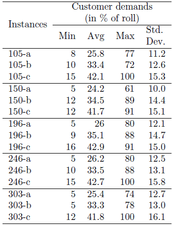
Table 2: Characteristics of the generated instances
From these values it can be noted that a city freighter trip cannot serve many customers. In addition, distances between customers are very small, so that one city freighter spends more time delivering customers than traveling. This justifies the modeling in which the traveled distance is only a secondary objective with respect to the number of vehicles used.
6.2.2 Comparison between conventional and mixed systems
The 15 generated data sets have been used to assess the two{tiered system. We compare the two following approaches:
delivering all customers directly from the CDC by using electric trucks having a capacity of 2 tons (20 containers). The corresponding optimization problem is a Vehicle Routing Problem with Time Windows (VRPTW). Vehicles can perform multiple trips provided there is no time windows conict between two consecutive trips. This problem has been solved with the ALNS algorithm of Pisinger and Ropke (2007b) that was developed and evaluated in Masson et al. (2012a).
delivering all customers through the two{tiered transportation system. The primary objective is to minimize the number of city freighters. The secondary objective is to minimize the distance traveled by city freighters. The distance traveled by buses is not accounted since their trips are planned beforehand and the buses would circulate with passengers even when no delivery of goods are planned.
Table 3 presents the numerical results obtained after a run time of 1 hour for each approach. The second and third columns indicate the number of used trucks and the traveled distance in the VRPTW. The fourth and fifth columns report the number of used city freighters and the traveled distance in the two{tiered system.
The results in the second and third columns show that the fleet of trucks remains stable with respect to the demand. On the other hand, the number of city freighters increases linearly with the number of customers but it remains close to the number of trucks. When the average demand increases, the distance traveled by trucks does not always increase, whereas this increase is significant for city freighters. This can be explained by the di
erence of capacity of the vehicles. Indeed, truck capacity is, in general, underutilized. On the contrary, city freighters have a small capacity. When the average demand increases, the average number of customers served in a trip decreases and a city freighter must return more frequently to a bus stop to load a new container.

Table 3: Comparison between the VRPTW and the two{tiered system
This analysis is confirmed by Table 4, which reports the utilization of vehicles. Values in the second column indicate the average load carried by trucks in the VRPTW approach. These values are computed as a ratio between the total load carried by trucks and their capacity. Since trucks can perform multiple trips, this ratio may exceed 1. Column three reports the same ratio for city freighters. The last two columns represent the number of used containers (number of trips) and their average fill ratSSe (in %).

Table 4: Vehicles fill rates
The table shows major differences between both systems. In the VRPTW, each truck is filled once or twice per day at the CDC and performs a route with many customers. In the two-tiered system, a city freighter performs many routes containing only a few customers. This highlights that an efficient transshipment of containers from buses to city freighters is a key factor in the transportation system performance. In addition, the risk related to a bad synchronization between a city freighter and a bus is high. The number of containers in column 4 is computed with the assumption that transportation is decoupled from order picking operations. Hence, the containers are already available and filled with goods when the first bus arrives at the CDC. Under this assumption, each roll can be used only once a day. An improvement would consist in picking orders during the day. This would make it possible to reuse empty containers coming back to the CDC, which would reduce the initial investment in term of containers. Considering the reverse flow of empty containers returning back to the CDC is left for further research.
Finally, Table 5 measures the impact of the two{tiered system on the existing infrastructure. Columns 2 to 7 represent the number of containers unloaded from the buses at bus stops T1 to T6.

Table 5: Practical use of bus stops
Bus stops T3 and T4 are located close to a large number of customers, so that 60% of the transshipments are operated at these stops. Hopefully, the model imposes a limit Qs on the number of containers that can be simultaneously transshipped. Thus, there is no congestion issue at bus stops. On the contrary, the utilization of bus stops T1, T2 and T5 is scarce, which is not a problem since no expensive investment is required here to modify the existing infrastructure. Note that the algorithm proposed in this paper can be easily used to run simulations and select a subset of transshipment locations, possibly with a small storage capacity in order to reduce risks related to synchronization issues.
7 Conclusion
In this paper we introduced and modeled the Mixed Urban Transportation Problem. We proposed several algorithms that contribute to its solution. In particular, we proposed an Adaptive Large Neighborhood Search algorithm to minimize the number of vehicles required. We underlined the difficulty of checking temporal constraints in a two-echelon multi-modal problem in which the first echelon is already scheduled. We proposed a heuristic to solve this feasibility problem. The model can be easily up-scaled, considering several bus lines, several CDCs and the possibility to mix the fleet of trucks and city freighters.
From the modeling and optimization point of view, many perspectives and interesting topics can be considered for further research, including: the exact solving of the MUTP and of its feasibility problem (RCAP), the integration of packing constraints when assigning orders to trips, the integration of the reverse flow of empty containers, the modeling and optimization of accurate operating and logistics costs. In this paper we considered a pure deterministic data. In practice, there are several causes of uncertainty: demand Crainic et al. (2012a), transportation and delivery times and in bus capacity. Mendoza (2011)
References
Baldacci, R., Bartolini, E., Mingozzi, A., 2011. An exact algorithm for the pickup and delivery problem with time windows. Operations Research 59 (2), 414-426.
Cattaruzza, D., Absi, N., Feillet, D., Guyon, O., Libeaut, X., August 2013. The multi trip vehicle routing problem with time windows and release dates. In: Proceedings of the 10th Metaheuristics International Conference (MIC 2013). pp. 1-10.
Cordeau, J.-F., Desaulniers, G., Desrosiers, J., Solomon, M., Soumis, F., 2002. VRP with time windows. In: Toth, P., Vigo, D. (Eds.), The Vehicle Routing Problem. Society Industrial and Applied Mathematics, pp. 157-193.
Cortes, C. E., Jayakrishnan, R., 2002. Design and operational concepts of high-coverage point-topoint transit system. Transportation Research Record 1783, 178-187.
Cortes, C. E., Matamala, M., Contardo, C., 2010. The pickup and delivery problem with transfers: Formulation and a branch-and-cut solution method. European Journal of Operational Research 200 (3), 711-724.
Crainic, T., Errico, F., Rei, W., Ricciardi, N., 2012a. Modeling demand uncertainty in two-tiered city logistics planning. Tech. rep., Publication CIRRELT-2012-65, Centre interuniversitaire defrecherche sur les reseaux d'entreprise, la logistique et le transport, Universite de Montreal, Montreal, QC, Canada.
Crainic, T. G., Gajpal, Y., Gendreau, M., 2012b. Multi-zone multi-trip vehicle routing problem with time windows. Tech. rep., CIRRELT-2012-36.
Crainic, T. G., Mancini, S., Perboli, G., Tadei, R., 2011. Multi-start heuristics for the twoechelon vehicle routing problem. In: Merz, P., Hao, J.-K. (Eds.), Evolutionary Computation in Combinatorial Optimization. Vol. 6622 of Lecture Notes in Computer Science. Springer Berlin Heidelberg, pp. 179-190.
Crainic, T. G., N., R., Storchi, G., 2009. Models for evaluation and planning city logistics systems. Transportation Science 43 (4), 432-454.
Crainic, T. G., Perboli, G., Mancini, S., Tadei, R., 2010. Two-echelon vehicle routing problem: A satellite location analysis. Procedia - Social and Behavioral Sciences 2 (3), 5944 - 5955.
Dueck, G., January 1993. New optimization heuristics: The great deluge algorithm and the record-to-record travel. Journal of Computational Physics 104, 86-92.
European Commission, Directorate-General for Energy and Transport, 2007. Towards a New Culture for Urban Mobility. Ofice for Oficial Publications of the European Communities.
Feillet, D., 2010. A tutorial on column generation and branch-and-price for vehicle routing problems. 4OR 8 (4), 407-424.
Feillet, D., Dejax, P., Gendreau, M., Gueguen, C., 2004. An exact algorithm for the elementary shortest path problem with resource constraints: Application to some vehicle routing problems. Networks 44 (3), 216-229.
Fugenschuh, A., 2009. Solving a school bus scheduling problem with integer programming. European Journal of Operational Research 193 (3), 867-884.
Gortz, I. L., Nagarajan, V., Ravi, R., 2009. Minimum makespan multi-vehicle dial-a-ride. In: Proceedings of the 17th ESA, Copenhagen, Denmark. Lecture Notes in CS. Vol. 5757. pp. 540-552.
Hemmelmayr, V. C., Cordeau, J.-F., Crainic, T. G., 2012. An adaptive large neighborhood search heuristic for two-echelon vehicle routing problems arising in city logistics. Computers & Operations Research 39(12), 3215-3228.
Jepsen, M., Spoorendonk, S., Ropke, S., Mar. 2012. A Branch-and-Cut Algorithm for the Symmetric Two-Echelon Capacitated Vehicle Routing Problem. Transportation Science 47 (1), 23-37.
Kerivin, H. L. M., Lacroix, M., Mahjoub, A. R., Quilliot, A., 2008. The splittable pickup and delivery problem with reloads. European Journal of Industrial Engineering 2 (2), 112-133.
Kirkpatrick, S., Gelatt, C. D., Vecchi, M. P., 1983. Optimization by simulated annealing. Science 220, 671-680.
Masson, R., Lehuede, F., Peton, O., 2012a. An adaptive large neighborhood search for the pickup and delivery problem with transfers. Transportation Science articles in advance, 1-12.
Masson, R., Lehuede, F., Peton, O., 2012b. The dial-a-ride problem with transfers. Computers and Operations Research submitted.
Masson, R., Lehuede, F., Peton, O., 2012c. Simple temporal problems in route scheduling for the dial-a-ride problem with transfers. In: Beldiceanu, N., Jussien, N., Pinson, E. (Eds.), Integration of AI and OR Techniques in Constraint Programming for Combinatorial Optimization Problems. Vol.7298 of LNCS. Springer, pp. 275-291.
Masson, R., Lehuede, F., Peton, O., Sep. 2013a. Efficient feasibility testing for request insertion in the Pickup and Delivery Problem with Transfers. Operations Research Letters 41 (3), 211-215.
Masson, R., Ropke, S., Lehuede, F., Peton, O., 2013b. A branch-and-cut-and-price for the pickup and delivery problem with shuttles routes. European Journal of Operational Research submitted. Mendoza, J. E., 2011. Solving real-world vehicle routing problems in uncertain environments. 4OR 9 (3), 321-324.
Mitrovic-Minic, S., Laporte, G., 2006. The pickup and delivery problem with time windows and transshipment. INFOR 44 (3), 217-228.
Nguyen, P., Crainic, T., Toulouse, M., 2013. A tabu search for time-dependent multi-zone multitrip vehicle routing problem with time windows. European Journal of Operational Research 231 (1), 43-56.
Perboli, G., Tadei, R., 2010. New families of valid inequalities for the two-echelon vehicle routing problem. Electronic Notes in Discrete Mathematics 36, 639-646.
Perboli, G., Tadei, R., Vigo, D., 2011. The two-echelon capacitated vehicle routing problem: Models and math-based heuristics. Transportation Science 45 (3), 364-380.
Petersen, H. L., Ropke, S., 2011. The pickup and delivery problem with cross-docking opportunity. In: Proceedings of the Second international conference on Computational logistics. ICCL'11. Springer-Verlag, Berlin, Heidelberg, pp. 101-113.
Pisinger, D., Ropke, S., 2007a. A general heuristic for vehicle routing problems. Computers and Operations Research 34 (8), 2403-2435.
Pisinger, D., Ropke, S., 2007b. A general heuristic for vehicle routing problems. Computers & Operations Research 34 (8), 2403-2435.
Pisinger, D., Ropke, S., 2010. Large neighborhood search. In: Gendreau, M., Potvin, J.-Y. (Eds.), Handbook of Metaheuristics. Vol. 146 of International Series in Operations Research & Management Science. Springer US, pp. 399-419.
Qu, Y., Bard, J. F., 2012. A GRASP with adaptive large neighborhood search for pickup and delivery problems with transshipment. Computers & Operations Research 39 (10), 2439-2456.
Roberti, R., Jun. 2012. Exact algorithms for different classes of vehicle routing problems. Ph.D. thesis, University of Bologna. Ropke, S., Cordeau, J.-F., 2009. Branch and Cut and Price for the Pickup and Delivery Problem with Time Windows. Transportation Science 43 (3), 267-286.
Ropke, S., Pisinger, D., 2006a. An adaptive large neighborhood search heuristic for the pickup and delivery problem with time windows. Transportation Science 40, 455-472.
Ropke, S., Pisinger, D., 2006b. A unified heuristic for a large class of vehicle routing problems with backhauls. European Journal of Operational Research 171 (3), 750-775.
Savelsbergh, M. W. P., 1992. The vehicle routing problem with time windows: Minimizing route duration. ORSA Journal on Computing 4 (2), 146-154.
Schrimpf, G., Schneider, J., Stamm-Wilbrandt, H., Dueck, G., 2000. Record breaking optimization results using the ruin and recreate principle. Journal of Computational Physics 159, 139-171.
Shang, J. S., Cuff, C. K., 1996. Multicriteria pickup and delivery problem with transfer opportunity. Computers & Industrial Engineering 30 (4), 631-645.
Shaw, P., 1998. Using constraint programming and local search methods to solve vehicle routing problems. In: Proceedings of the 4th International Conference on Principles and Practice of Constraint Programming. pp. 417-431.
Stein, D., 1978. Scheduling dial{a{ride transportation systems. Transportation Science 12, 232-249.
Trentini, A., Campi, A., Malhene, N., Boscacci, F., 2011. Shared passengers & goods urban transport solutions: new ideas for milan through en international comparison. Territorio 59, 38-44.
Trentini, A., Malhene, N., 2010. Toward a shared urban transport system ensuring passengers & goods cohabitation. TeMA 3 (2).