A Comparative Analysis of SIFT, SURF, KAZE, AKAZE, ORB, and BRISK
Abstract. Image registration is the process of matching, aligning and overlaying two or more images of a scene, which are captured from different viewpoints. It is extensively used in numerous vision based applications. Image registration has five main stages: Feature Detection and Description; Feature Matching; Outlier Rejection; Derivation of Transformation Function; and Image Reconstruction. Timing and accuracy of feature-based Image Registration mainly depend on computational efficiency and robustness of the selected feature-detector-descriptor, respectively. Therefore, choice of feature-detector-descriptor is a critical decision in feature-matching applications. This article presents a comprehensive comparison of SIFT, SURF, KAZE, AKAZE, ORB, and BRISK algorithms. It also elucidates a critical dilemma: Which algorithm is more invariant to scale, rotation and viewpoint changes? To investigate this problem, image matching has been performed with these features to match the scaled versions (5% to 500%), rotated versions (0° to 360°), and perspective-transformed versions of standard images with the original ones. Experiments have been conducted on diverse images taken from benchmark datasets: University of OXFORD, MATLAB, VLFeat, and OpenCV. Nearest-Neighbor-Distance-Ratio has been used as the feature-matching strategy while RANSAChas been applied for rejecting outliers and fitting the transformation models. Results are presented in terms of quantitative comparison, feature-detection-description time, feature-matching time, time of outlier-rejection and model fitting, repeatability, and error in recovered results as compared to the ground-truths. SIFT and BRISK are found to be the most accurate algorithms while ORB and BRISK are most efficient. The article comprises rich information that will be very useful formaking important decisions in vision based applications and main aim of this work is to set a benchmark for researchers, regardless of any particular area.
Keywords: SIFT; SURF; KAZE; AKAZE; ORB; BRISK; RANSAC; nearest neighbor distance ratio; feature detection; feature matching; image registration; scale invariance; rotation invariance; affine invariance; image matching; mosaicing
I. Introduction
Image matching is the cornerstone of many computer and machine vision applications specially: Robot Navigation, Pose Estimation [1], Visual Odometry [2], [3]; Visual Simultaneous Localization and Mapping [4], [5]; Object Detection, Object Tracking, Augmented Reality [6], Image Mosaicing, and Panorama Stitching [7]. Pose estimation is performed by deriving the perspective transform for the image captured at final pose with respect to the image captured at initial pose.
Visual odometry is the measurement of distance covered by a mobile system on the basis of visual information. Vision based Simultaneous Localization and Mapping deals with localizing a mobile agent in an environment while mapping its surroundings simultaneously. Object detection and tracking is based on detection and matching of common features between object’s image and the scene. Image stitching or mosaicing is the process of generating a large-scale consolidated image from multiple small-scale overlapping images. It is widely applied in aerial, marine and satellite imagery to yield a continuous single picture of subject environments. Panorama generation software provided in mobile phones and digital cameras is another major application of mosaicing. All these applications require presence of some overlapping region (typically more than 30%) between any two successive images for matching.
Five main stages of image registration are: Feature Detection and Description; Feature Matching; Outlier Rejection; Derivation of Transformation Function; and Image Reconstruction. A feature-detector is an algorithm that detects feature-points (also called interest-points or key-points) in an image [8]. Features are generally detected in the form of corners, blobs, edges, junctions, lines etc. The detected features are subsequently described in logically different ways on the basis of unique patterns possessed by their neighboring pixels. This process is called feature description as it describes each feature by assigning it a distinctive identity which enables their effective recognition for matching. Some feature-detectors are readily available with their designated feature description algorithm while others exist individually. However the individual feature-detectors can be paired with several types of pertinent feature-descriptors. SIFT, SURF, KAZE, AKAZE, ORB, and BRISK are among the fundamental scale, rotation and affine invariant feature-detectors, each having a designated feature-descriptor and possessing its own merits and demerits. Therefore, the term feature-detector-
descriptor
will be used for these algorithms in this paper.
After feature-detection-description, feature-matching is performed by using L1-norm or L2-norm for string based descriptors (SIFT, SURF, KAZE etc.) and Hamming distance for binary descriptors (AKAZE, ORB, BRISK etc.). Different matching strategies can be adopted for matching features like Threshold based matching; Nearest Neighbor; Nearest Neighbor Distance Ratio etc. each having its own strengths and weaknesses [9]. Incorrect matches (or outliers) cannot be completely avoided in the feature-matching stage, thus another phase of outlier-rejection is mandatory for accurate fitting of transformation model. Random Sample Consensus (RANSAC) [10], M-estimator Sample Consensus (MSAC) [11], and Progressive Sample Consensus (PROSAC) [12] are some of the robust probabilistic methods used for removing the outliers from matched features and fitting the transformation function (in terms of homography matrix). This matrix provides the perspective transform of second image with respect to the first (reference image). Image reconstruction is then performed on the basis of the derived transformation function to align the second image with respect to the first. The reconstructed version of second image is then overlaid in front of the reference image until all matched feature-points are overlapped. This large consolidated version of smaller images is called a mosaic or stitched image. Fig. 1 shows the generic process of feature based image registration.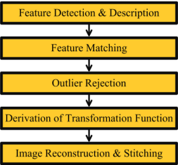
In this article, SIFT (blobs) [13], SURF (blobs) [14], KAZE (blobs) [15], AKAZE (blobs) [16], ORB (corners) [17], and BRISK (corners) [18] algorithms are compared for image matching and registration. The performance of feature-detector-descriptors is further evaluated to investigate: Which is more invariant to scale, rotation and affine changes? To inspect this problem, image matching has been done with these feature-detector-descriptors to match the synthetically scaled versions (5% to 500%) and synthetically rotated versions (0° to 360°) of different images with their original versions. To investigate viewpoint or affine invariance, image matching has been performed for the Graffiti sequence and Wall sequence. Experiments have been conducted on diverse images taken from the well-known datasets of University of OXFORD [19], MATLAB, VLFeat, and OpenCV. Nearest Neighbor Distance Ratio has been applied as the feature-matching strategy with Brute-force search algorithm while RANSAC has been applied for fitting the image transformation models (in the form of homography matrices) and for rejecting the outliers. The experimental results are presented in the form of quantitative comparison, feature-detection-description time, feature-matching time, outlier-rejection and model fitting time, repeatability, and error in recovered results as compared to the ground-truth values. This article will act as a stepping stone in the selection of most suitable feature-detector-descriptor with required strengths for feature based applications in the domain of computer vision and machine vision. As far as our knowledge is concerned, there exists no such research that so exhaustively evaluates these fundamental feature-detector-descriptors over a diverse set of images for the discussed problems.
II. Literature review
A. Performance Evaluations of Detectors & Descriptors
Literature review for this article is based on many high quality research articles that provide comparison results of various types of feature-detectors and feature-descriptors. K. Mikolajczyk and C. Schmid evaluated the performance of local feature-descriptors (SIFT, PCA-SIFT, Steerable Filters, Complex Filters, GLOH etc.) over a diverse dataset for different image transformations (rotation, rotation combined with zoom, viewpoint changes, image blur, JPEG compression, and light changes) [9]. However, scale changes that have been evaluated in this article lie only in the range of 200% to 250%. S. Urban and M. Weinmann compared different feature-detector-descriptor combinations (like SIFT, SURF, ORB, SURF-BinBoost, and AKAZE-MSURF) for registration of point clouds obtained through terrestrial laser scanning in [20]. In [21], S. Gauglitz et al. evaluated different feature-detectors (Harris Corner Detector, Difference of Gaussians, Good Features to Track, Fast Hessian, FAST, CenSurE) and feature-descriptors (Image patch, SIFT, SURF, Randomized Trees, and Ferns) for visual tracking but no quantitative comparison and no evaluation of rotation and scale invariance property is performed. Z. Pusztai and L. Hajder provide a quantitative comparison of various feature-detectors available in OpenCV 3.0 (BRISK, FAST, GFTT, KAZE, MSER, ORB, SIFT, STAR, SURF, AGAST, and AKAZE) for viewpoint changes on four image data sequences in [22] but no comparison of computational timings is present. H. J. Chien et al. compare SIFT, SURF, ORB, and AKAZE features for monocular visual odometry by using the KITTI benchmark dataset in [23], however there is no explicit in-depth comparison for rotation, scale and affine invariance property of the feature-detectors. N. Y. Khan et al. evaluated the performance of SIFT and SURF against various types of image deformations using threshold based feature-matching [24]. However, no quantitative comparison is performed and evaluation of in-depth scale invariance property is missing.
B. SIFT
D. G. Lowe introduced Scale Invariant Feature Transform (SIFT) in 2004 [13], which is the most renowned feature-detection-description algorithm. SIFT detector is based on Difference-of-Gaussians (DoG) operator which is an approximation of Laplacian-of-Gaussian (LoG). Feature-points are detected by searching local maxima using DoG at various scales of the subject images. The description method extracts a 16x16 neighborhood around each detected feature and further segments the region into sub-blocks, rendering a total of 128 bin values. SIFT is robustly invariant to image rotations, scale, and limited affine variations but its main drawback is high computational cost. Equation (1) shows the convolution of difference of two Gaussians (computed at different scales) with image I(x, y).

Where G represents the Gaussian function.
C. SURF
H. Bay et al. presented Speeded Up Robust Features (SURF) in 2008 [14], which also relies on Gaussian scale space analysis of images. SURF detector is based on determinant of Hessian Matrix and it exploits integral images to improve feature-detection speed. The 64 bin descriptor of SURF describes each detected feature with a distribution of Haar wavelet responses within certain neighborhood. SURF features are invariant to rotation and scale but they have little affine invariance. However, the descriptor can be extended to 128 bin values in order to deal with larger viewpoint changes. The main advantage of SURF over SIFT is its low computational cost. Equation (2) represents the Hessian Matrix in point x = (x, y) at scale σ.

Where Lxx(x, σ) is the convolution of Gaussian second order derivative with the image I in point x, and similarly for Lxy (x, σ) and Lyy(x, σ).
D. KAZE
P. F. Alcantarilla et al. put forward KAZE features in 2012 that exploit non-linear scale space through non-linear diffusion filtering [15]. This makes blurring in images locally adaptive to feature-points, thus reducing noise and simultaneously retaining the boundaries of regions in subject images. KAZE detector is based on scale normalized determinant of Hessian Matrix which is computed at multiple scale levels. The maxima of detector response are picked up as feature-points using a moving window. Feature description introduces the property of rotation invariance by finding dominant orientation in a circular neighborhood around each detected feature. KAZE features are invariant to rotation, scale, limited affine and have more distinctiveness at varying scales with the cost of moderate increase in computational time. Equation (3) shows the standard nonlinear diffusion formula.

Where c is conductivity function, div is divergence, ∇ is gradient operator and L is image luminance.
E. AKAZE
P. F. Alcantarilla et al. presented Accelerated-KAZE (AKAZE) algorithm in 2013 [16], which is also based on non-linear diffusion filtering like KAZE but its non-linear scale spaces are constructed using a computationally efficient framework called Fast Explicit Diffusion (FED). The AKAZE detector is based on the determinant of Hessian Matrix. Rotation invariance quality is improved using Scharr filters. Maxima of the detector responses in spatial locations are picked up as feature-points. Descriptor of AKAZE is based on Modified Local Difference Binary (MLDB) algorithm which is also highly efficient. AKAZE features are invariant to scale, rotation, limited affine and have more distinctiveness at varying scales because of nonlinear scale spaces.
F. ORBM
E. Rublee et al. introduced Oriented FAST and Rotated BRIEF (ORB) in 2011 [17]. ORB algorithm is a blend of modified FAST (Features from Accelerated Segment Test) [25] detection and direction-normalized BRIEF (Binary Robust Independent Elementary Features) [26] description methods. FAST corners are detected in each layer of the scale pyramid and cornerness of detected points is evaluated using Harris Corner score to filter out top quality points. As BRIEF description method is highly unstable with rotation, thus a modified version of BRIEF descriptor has been employed. ORB features are invariant to scale, rotation and limited affine changes.
G. BRISK
S. Leutenegger et al. put forward Binary Robust Invariant Scalable Keypoints (BRISK) in 2011 [18], which detects corners using AGAST algorithm and filters them with FAST Corner score while searching for maxima in the scale space pyramid. BRISK description is based on identifying the characteristic direction of each feature for achieving rotation invariance. To cater illumination invariance results of simple brightness tests are also concatenated and the descriptor is constructed as a binary string. BRISK features are invariant to scale, rotation, and limited affine changes.
III. Experiments & Results
A. Experimental Setup
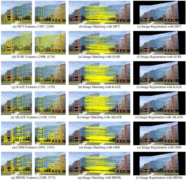
MATLAB-2017a with OpenCV 3.3 has been used for performing the experiments presented in this article. Specifications of the computer system used are: Intel(R) Core(TM) i5–4670 CPU @ 3.40 GHz, 6 MB Cache and 8.00 GB RAM. SURF(64D) , SURF(128D), ORB(1000), and BRISK(1000) represent SURF with 64-Floats descriptor, extended SURF with 128-Floats descriptor, bounded ORB and BRISK detectors with an upper bound to detect only up to best 1000 feature-points, respectively. Table I shows OpenCV’s objects used for the feature-detector-descriptors. All remaining parameters are used as OpenCV’s default.
| Algorithm | OpenCV Object | Descripror Size |
|---|---|---|
| SIFT | cv.SIFT('ConstrastThreshold',0.04,'Sigma',1.6) | 128 bytes |
| SURF(128D) | cv.SURF('Extended',true,'HessianThreshold',100) | 128 Floats |
| SURF(64D) | cv.SURF('HessianThreshold',100) | 64 Floats |
| KAZE | cv.KAZE('NOctaveLayers',3,'Extended',true) | 128 Bytes |
| AKAZE | cv.AKAZE('NOctaveLayers',3) | 61 Bytes |
| ORB | cv.ORB('MaxFeatures',100000) | 32 Bytes |
| ORB(1000) | cv.ORB('MaxFeatures',1000) | 32 Bytes |
| BRISK | cv.BRISK() | 64 Bytes |
| BRISK(1000) | cv.BRISK(); cv.KeyPointsFilter.retainBest(features,1000) | 64 Bytes |
B. Datasets
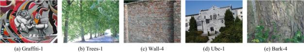
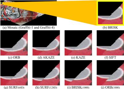
Two datasets have been used for this research. Dataset-A (see Fig. 2) is prepared by selecting 6 image pairs of diverse scenes from different benchmark datasets. Building and Bricks images shown in Fig. 2(a) and Fig. 2(d), respectively, are selected from the vision toolbox of MATLAB. The image pair of Mountains shown in Fig. 2(g) is taken from the test data of OpenCV. Graffiti-1 and Graffiti-4 shown in Fig. 2(j) are picked from University of OXFORD’s Affine Covariant Regions Datasets [19]. Image pairs of Roofs and River shown in Fig. 2(m) and Fig. 2(p), respectively, are taken from the data of VLFeat library. Dataset-B (see Fig. 3) is based on 5 images chosen from University of OXFORD’s Affine Covariant Regions Datasets. Dataset-A has been used to compare different aspects of feature-detector-descriptors for image registration process while Dataset-B has been used to investigate scale, and rotation invariance capability of the feature-detector-descriptors. Furthermore, to investigate affine invariance, Graffiti sequence and Wall sequence from the Affine Covariant Regions Datasets have been exploited.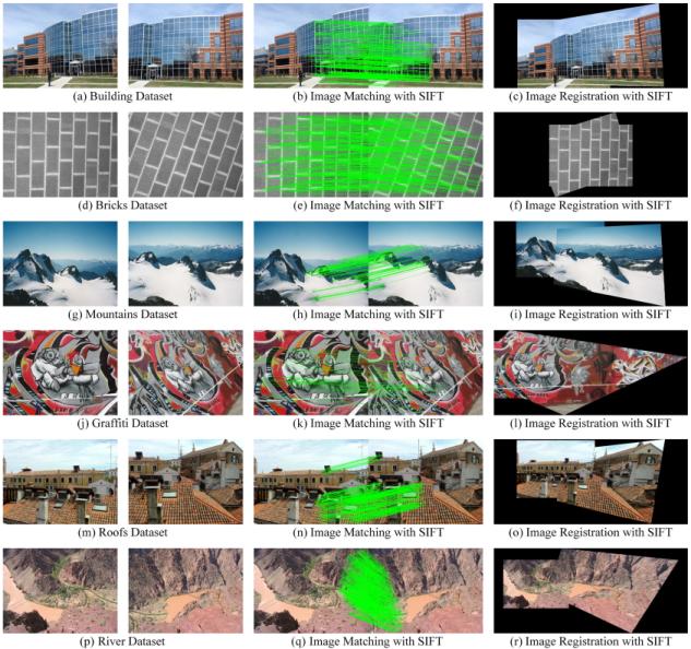
C. Ground-truths
Ground-truth values for image transformations have been used to calculate and demonstrate error in the recovered results with each feature-detector-descriptor. For evaluating scale and rotation invariance, ground-truths have been synthetically generated for each image in Dataset-B by resizing and rotating it to known values of scale (5% to 500%) and rotation (0° to 360°). Bicubic interpolation has been adopted for scaling and rotating images since it is the most accurate interpolation method which retains image quality in the transformation process. To investigate affine invariance the benchmark ground-truths provided in Affine Covariant Regions Datasets for Graffiti and Wall sequences have been used.
D. Matching Strategy
The feature-matching strategy adopted for experiments is based on Nearest Neighbor Distance Ratio (NNDR) which was used by D.G. Lowe for matching SIFT features in [13] and by K. Mikolajczyk in [9]. In this matching scheme, the nearest neighbor and the second nearest neighbor for each feature-descriptor (from the first feature set) are searched (in the second feature set). Subsequently, ratio of nearest neighbor to the second nearest neighbor is calculated for each feature-descriptor and a certain threshold ratio is set to filter out the preferred matches. This threshold ratio is kept as 0.7 for the experimental results presented in this article. L1-norm (also called Least Absolute Deviations) has been used for matching the descriptors of SIFT, SURF, and KAZE while Hamming distance has been used for matching the descriptors of AKAZE, ORB, and BRISK.
E. Outlier Rejection & Homography Calculation
RANSAC algorithm with 2000 iterations and 99.5% confidence has been applied to reject the outliers and to find the Homography Matrix. It is a 3x3 matrix that represents a set of equations which satisfy the transformation function from the first image to the second.
F. Repeatability
Repeatability of a feature-detector is the percentage of detected features that survive photometric or geometric transformations in an image [27]. Repeatability is not related with the descriptors and only depends on performance of the feature-detection part of feature-detection-description algorithms. It is calculated on the basis of the overlapping (intersecting) region in the subject image pair. A feature-detector with higher repeatability for a particular transformation is considered robust than others, particularly for that type of transformation.
G. Demonstration of Results
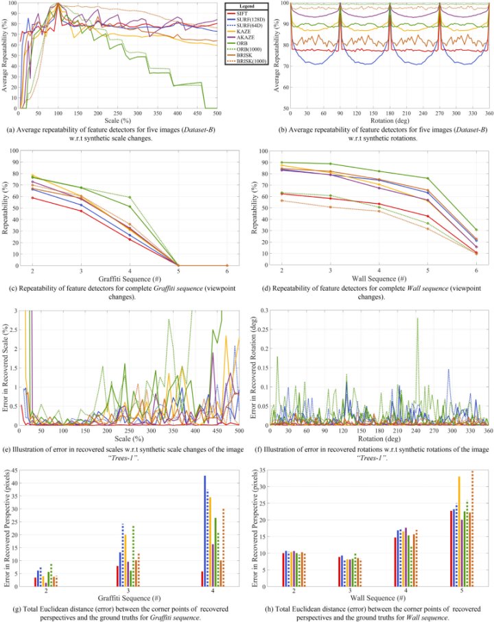
Table II shows the results of quantitative comparison and computational costs of the feature-detector-descriptors for image matching. Each timing value presented in the table is the average of 100 measurements (to minimize errors which arise because of processing glitches). The synthetically generated scale / rotation transformations for the images of Dataset-B and the readily available ground-truth affine transformations for Graffiti / Wall sequences are recovered by performing image matching with each feature-detector-descriptor. Average repeatabilities of each feature-detector (for 5 images of Dataset-B) to investigate the trend of their strengths / weaknesses are presented in Fig. 6(a) and Fig. 6(b) for scale and rotation changes, respectively. Fig. 6(c) and Fig. 6(d) show the repeatability of feature-detectors for viewpoint changes using benchmark datasets. Fig. 6(e) and Fig. 6(f) exhibit the error in recovered scales and rotations for all the feature-detector-descriptors in terms of percentage and degree, respectively. To compute errors in affine transformations, the images of Graffiti and Wall sequences were first warped according to the ground-truth homographies as well as the recovered homographies. Afterwards, Euclidean distance has been calculated individually for each corner point of the recovered image with respect to its corresponding corner point (in the ground-truth image). Fig. 6(g) and Fig. 6(h) illustrate the projection error in recovered affine transformations as the sum of 4 Euclidean distances for Graffiti and Wall sequences, respectively. The error is represented in terms of pixels. Equation (4) shows the Euclidean distance D(P, Q)
between two corresponding corners P(xp, yp) and Q(xq, yq).
| Algorithm | Features Detected in the Image Pairs | Features Matched | Outliers Rejected | Features Detection & Description Time (s) | Feature Matching Time (s) | Outlier Rejection & Homography Calculation Time (s) | Total Image Matching Time (s) | ||
|---|---|---|---|---|---|---|---|---|---|
| 1st Image | 2nd Image | 1st Image | 2nd Image | ||||||
| Building Dataset (Image Pair # 1) | |||||||||
| SIFT | 1907 | 2209 | 384 | 51 | 0.1812 | 0.1980 | 0.1337 | 0.0057 | 0.5186 |
| SURF (128D) | 3988 | 4570 | 319 | 58 | 0.1657 | 0.1786 | 0.5439 | 0.0058 | 0.8940 |
| SURF (64D) | 3988 | 4570 | 612 | 73 | 0.1625 | 0.1734 | 0.2956 | 0.0052 | 0.6367 |
| KAZE | 1291 | 1359 | 465 | 26 | 0.2145 | 0.2113 | 0.0613 | 0.0053 | 0.4924 |
| AKAZE | 1458 | 1554 | 475 | 36 | 0.0695 | 0.0715 | 0.0307 | 0.0055 | 0.1772 |
| ORB | 5095 | 5345 | 854 | 149 | 0.0213 | 0.0220 | 0.1586 | 0.0067 | 0.2086 |
| ORB (1000) | 1000 | 1000 | 237 | 21 | 0.0103 | 0.0101 | 0.0138 | 0.0049 | 0.0391 |
| BRISK | 3288 | 3575 | 481 | 47 | 0.0533 | 0.0565 | 0.1236 | 0.0056 | 0.2390 |
| BRISK (1000) | 1000 | 1000 | 190 | 33 | 0.0188 | 0.0191 | 0.0158 | 0.0049 | 0.0586 |
| Bricks Dataset (Image Pair # 2) | |||||||||
| SIFT | 1404 | 1405 | 427 | 16 | 0.1571 | 0.1585 | 0.0680 | 0.0053 | 0.3889 |
| SURF (128D) | 2855 | 2332 | 140 | 34 | 0.1337 | 0.1191 | 0.2066 | 0.0051 | 0.4645 |
| SURF (64D) | 2855 | 2332 | 327 | 63 | 0.1307 | 0.1137 | 0.1173 | 0.0055 | 0.3672 |
| KAZE | 366 | 705 | 88 | 6 | 0.1930 | 0.1988 | 0.0105 | 0.0047 | 0.4070 |
| AKAZE | 278 | 289 | 153 | 9 | 0.0541 | 0.0536 | 0.0037 | 0.0049 | 0.1163 |
| ORB | 978 | 942 | 323 | 17 | 0.0075 | 0.0079 | 0.0124 | 0.0049 | 0.0327 |
| ORB (1000) | 731 | 734 | 240 | 32 | 0.0067 | 0.0073 | 0.0088 | 0.0050 | 0.0278 |
| BRISK | 796 | 752 | 285 | 18 | 0.0146 | 0.0144 | 0.0119 | 0.0049 | 0.0458 |
| BRISK (1000) | 796 | 752 | 285 | 18 | 0.0146 | 0.0144 | 0.0119 | 0.0049 | 0.0458 |
| Mountain Dataset (Image Pair # 3) | |||||||||
| SIFT | 1867 | 2033 | 170 | 45 | 0.1943 | 0.2017 | 0.1197 | 0.0047 | 0.5204 |
| SURF (128D) | 1890 | 2006 | 175 | 33 | 0.0979 | 0.1130 | 0.1208 | 0.0051 | 0.3368 |
| SURF (64D) | 1890 | 2006 | 227 | 62 | 0.0978 | 0.1113 | 0.0689 | 0.0053 | 0.2833 |
| KAZE | 972 | 971 | 131 | 20 | 0.2787 | 0.2826 | 0.0343 | 0.0050 | 0.6006 |
| AKAZE | 960 | 986 | 187 | 16 | 0.0841 | 0.0842 | 0.0151 | 0.0050 | 0.1884 |
| ORB | 4791 | 5006 | 340 | 78 | 0.0228 | 0.0236 | 0.1397 | 0.0052 | 0.1913 |
| ORB (1000) | 1000 | 1000 | 113 | 29 | 0.0118 | 0.0118 | 0.0117 | 0.0049 | 0.0402 |
| BRISK | 3153 | 3382 | 287 | 22 | 0.0520 | 0.0555 | 0.1083 | 0.0052 | 0.2210 |
| BRISK (1000) | 1000 | 1000 | 143 | 7 | 0.0201 | 0.0213 | 0.0160 | 0.0046 | 0.0620 |
| Graffiti Dataset (Image Pair # 4) | |||||||||
| SIFT | 2654 | 3698 | 99 | 51 | 0.2858 | 0.3382 | 0.2940 | 0.0073 | 0.9253 |
| SURF (128D) | 4802 | 5259 | 44 | 31 | 0.2166 | 0.2184 | 0.7399 | 0.0222 | 1.1971 |
| SURF (64D) | 4802 | 5259 | 62 | 42 | 0.2072 | 0.2142 | 0.3951 | 0.0169 | 0.8334 |
| KAZE | 2232 | 2302 | 30 | 9 | 0.3311 | 0.3337 | 0.1594 | 0.0052 | 0.8294 |
| AKAZE | 2064 | 2205 | 23 | 13 | 0.1158 | 0.1185 | 0.0491 | 0.0081 | 0.2915 |
| ORB | 5527 | 7517 | 38 | 22 | 0.0277 | 0.0341 | 0.2129 | 0.0083 | 0.2830 |
| ORB (1000) | 1000 | 1000 | 16 | 7 | 0.0146 | 0.0157 | 0.0114 | 0.0059 | 0.0476 |
| BRISK | 3507 | 5191 | 54 | 22 | 0.0669 | 0.0953 | 0.1687 | 0.0077 | 0.3386 |
| BRISK (1000) | 1000 | 1000 | 18 | 10 | 0.0227 | 0.0239 | 0.0143 | 0.0073 | 0.0682 |
| Roofs Dataset (Image Pair # 5) | |||||||||
| SIFT | 2303 | 3550 | 423 | 154 | 0.1983 | 0.2665 | 0.2475 | 0.0063 | 0.7186 |
| SURF (128D) | 2938 | 3830 | 171 | 95 | 0.1173 | 0.1523 | 0.3349 | 0.0084 | 0.6129 |
| SURF (64D) | 2938 | 3830 | 247 | 143 | 0.1165 | 0.1504 | 0.1847 | 0.0090 | 0.4606 |
| KAZE | 1260 | 1736 | 172 | 85 | 0.2119 | 0.2265 | 0.0710 | 0.0068 | 0.5162 |
| AKAZE | 1287 | 1987 | 175 | 59 | 0.0686 | 0.0806 | 0.0294 | 0.0053 | 0.1839 |
| ORB | 7660 | 11040 | 498 | 157 | 0.0296 | 0.0407 | 0.4131 | 0.0065 | 0.4899 |
| ORB (1000) | 1000 | 1000 | 91 | 32 | 0.0106 | 0.0113 | 0.0111 | 0.0055 | 0.0385 |
| BRISK | 5323 | 7683 | 436 | 207 | 0.0899 | 0.1260 | 0.3672 | 0.0074 | 0.5905 |
| BRISK (1000) | 1000 | 1000 | 90 | 44 | 0.0189 | 0.0199 | 0.0156 | 0.0069 | 0.0613 |
| River Dataset (Image Pair # 6) | |||||||||
| SIFT | 8619 | 9082 | 1322 | 192 | 0.6795 | 0.7083 | 2.2582 | 0.0092 | 3.6552 |
| SURF (128D) | 9434 | 10471 | 223 | 63 | 0.3768 | 0.4205 | 2.8521 | 0.0055 | 3.6549 |
| SURF (64D) | 9434 | 10471 | 386 | 66 | 0.3686 | 0.4091 | 1.4905 | 0.0049 | 2.2731 |
| KAZE | 2984 | 2891 | 391 | 78 | 0.5119 | 0.5115 | 0.2669 | 0.0059 | 1.2962 |
| AKAZE | 3751 | 3635 | 376 | 65 | 0.2048 | 0.1991 | 0.1341 | 0.0056 | 0.5436 |
| ORB | 34645 | 35118 | 2400 | 553 | 0.1219 | 0.1276 | 5.3813 | 0.0092 | 5.6400 |
| ORB (1000) | 1000 | 1000 | 40 | 6 | 0.0235 | 0.0235 | 0.0109 | 0.0046 | 0.0625 |
| BRISK | 23607 | 24278 | 1725 | 366 | 0.3813 | 0.4040 | 4.8117 | 0.0089 | 5.6059 |
| BRISK (1000) | 1000 | 1000 | 39 | 8 | 0.0251 | 0.0248 | 0.0155 | 0.0040 | 0.0694 |
| Mean Values for All Image Pairs | |||||||||
| SIFT | 3125.7 | 3662.8 | 470.8 | 84.8 | 0.2827 | 0.3119 | 0.5202 | 0.0064 | 1.1212 |
| SURF (128D) | 4317.8 | 4744.7 | 178.7 | 52.3 | 0.1847 | 0.2003 | 0.7997 | 0.0087 | 1.1934 |
| SURF (64D) | 4317.8 | 4744.7 | 310.2 | 74.8 | 0.1806 | 0.1954 | 0.4254 | 0.0078 | 0.8092 |
| KAZE | 1517.5 | 1660.7 | 212.8 | 37.3 | 0.2902 | 0.2941 | 0.1006 | 0.0055 | 0.6904 |
| AKAZE | 1633.0 | 1776.0 | 231.5 | 33.0 | 0.0995 | 0.1013 | 0.0437 | 0.0057 | 0.2502 |
| ORB | 9782.7 | 10828.0 | 742.2 | 162.7 | 0.0385 | 0.0427 | 1.0530 | 0.0068 | 1.1410 |
| ORB (1000) | 955.2 | 955.7 | 122.8 | 21.2 | 0.0129 | 0.0133 | 0.0113 | 0.0051 | 0.0426 |
| BRISK | 6612.3 | 7476.8 | 544.7 | 113.7 | 0.1097 | 0.1253 | 0.9319 | 0.0066 | 1.1735 |
| BRISK (1000) | 966.0 | 958.7 | 127.5 | 20.0 | 0.0200 | 0.0206 | 0.0149 | 0.0054 | 0.0609 |
IV. Important Findings
A. Quantitative Comparison:
- ORB detects the highest number of features (see Table II).
- BRISK is the runner-up as it detects more number of features than SIFT, SURF, KAZE, and AKAZE.
- SURF detects more features than SIFT.
- AKAZE generally detects more features than KAZE.
- KAZE detected least number of feature-points.
- For SURF(64D), more features are matched as compared to SURF(128D).
- SIFT and SURF features are detected in a scattered form generally all over the image and SURF features are denser than SIFT. ORB and BRISK features are more concentrated on corners.
B. Feature-Detection-Description Time
- KAZE has the highest computational cost for feature-detection-description (see Table III).
- Computational cost of SIFT is even less than half the cost of KAZE.
- ORB is the most efficient feature-detector-descriptor with least computational cost.
- BRISK is also computationally efficient but it is slightly expensive than ORB.
- SURF (128D) and SURF (64D) both are computationally efficient than SIFT (128D) (see Table III).
- AKAZE is computationally efficient than SIFT, SURF (128D) , SURF (64D) , and KAZE but expensive than ORB and BRISK.
| Algorithm | Mean Feature-Detection-Description Time per Point (μs) | Mean Feature Matching Time per Point (μs) | |
|---|---|---|---|
| 1st Images | 2nd Images | ||
| SIFT | 90.44 | 85.15 | 142.02 |
| SURF (128D) | 42.78 | 42.22 | 168.55 |
| SURF (64D) | 41.83 | 41.18 | 89.66 |
| KAZE | 191.24 | 177.09 | 60.58 |
| AKAZE | 60.93 | 57.04 | 24.61 |
| ORB | 3.94 | 3.94 | 97.25 |
| ORB (1000) | 13.51 | 13.92 | 11.82 |
| BRISK | 16.59 | 16.76 | 124.64 |
| BRISK (1000) | 20.70 | 21.49 | 15.42 |
C. Feature Matching Time:
- SURF(128D) has the highest computational cost for feature-matching while SIFT comes at the second place.
- SURF(64D) has less feature-matching cost as compared to SIFT. Which means that the feature-matching time for SURF(64D) is less than that of SIFT(128D) but the feature-matching time of SURF(128D) is more than that of SIFT(128D) .
- ORB and BRISK in unbounded state detect a large quantity of features due to which their feature-matching cost gets drastically increased. Table II shows that the feature-matching cost can be reduced by using their detectors in a bounded state i.e. ORB(1000) and BRISK(1000).
- ORB(1000) has the least feature-matching cost.
- Although KAZE has the highest cost for feature-detection-description, the computational cost of matching KAZE feature-descriptors is surprisingly lower than SIFT, SURF(128D) , SURF(64D) , ORB, and BRISK.
- The feature-matching cost of AKAZE is less than KAZE.
D. Outlier Rejection and Homography Fitting Time:
- The outlier-rejection and homography fitting time for all feature-detector-descriptors is more or less the same, though ORB(1000) and BRISK(1000) have taken least time.
E. Total Image Matching Time:
- ORB(1000) and BRISK(1000) provide fastest image matching.
- It is a general perception that SURF is computationally efficient than SIFT, but the experiments revealed that SURF(128D) algorithm takes more time than SIFT (128D) for the overall image matching process (see Table II).
- SURF(64D), on the contrary, takes less time than SIFT(128D) for image matching.
- Image matching time taken by KAZE is surprisingly less than SIFT, SURF(128D) , and even SURF(64D) (see Table II). This is due to the lower feature-matching cost of KAZE.
- The computational cost of feature-detection-description for ORB and BRISK (in unbounded state) is considerably low but the increased time for matching this large quantity of features lengthens their overall image matching time.
F. Repeatability:
- Repeatability of ORB for matching images remains stable and high as long as the scale of test image remains in the range of 60% to 150% with respect to the reference image but beyond this range, its repeatability drops considerably.
- ORB(1000) and BRISK(1000) have higher repeatability than ORB and BRISK for image rotations and up scaling. However, the case is reverse for down scaling (see Fig. 6(a)).
- Repeatability of SIFT, SURF, KAZE, AKAZE, and BRISK remains high for up scaling of images while in the case of down scaling, the repeatability of KAZE, AKAZE, and BRISK drops significantly. Repeatability of SIFT and SURF remains steady for scale variations but SURF’s plummets around 10% scale. SIFT’s repeatability has remained stable for down scaling to as low as 3% while the repeatabilities of others approach zero even at a scale of 15%.
- For image rotations, ORB(1000) , BRISK(1000), AKAZE, ORB, and KAZE have higher repeatabilities than SIFT and SURF.
- For affine changes, repeatabilities of ORB and BRISK are generally higher than others (see Fig. 6(c) and Fig. 6(d)).
G. Accuracy of Image Matching:
- SIFT is found to be the most accurate feature-detector-descriptor for scale, rotation and affine variations (overall).
- BRISK is at second position with respect to the accuracy for scale and rotation changes.
- AKAZE’s accuracy is comparable to BRISK for image rotations and scale variations in the range of 40% to 400%. Beyond this range its accuracy decreases.
- ORB(1000) is less accurate than BRISK(1000) for scale and rotation changes but both are comparable for affine changes.
- ORB(1000) and BRISK(1000) are less accurate than ORB and BRISK (see Fig. 5 and Fig. 6). These algorithms have a trade-off between quantity of features, feature-matching cost and the required accuracy of results.
- AKAZE is more accurate than KAZE for scale and affine variations. However, for rotation changes KAZE is more accurate than AKAZE
Conclusion
This article presents an exhaustive comparison of SIFT, SURF, KAZE, AKAZE, ORB, and BRISK feature-detector-descriptors. The experimental results provide rich information and various new insights that are valuable for making critical decisions in vision based applications. SIFT, SURF, and BRISK are found to be the most scale invariant feature detectors (on the basis of repeatability) that have survived wide spread scale variations. ORB is found to be least scale invariant. ORB(1000), BRISK(1000), and AKAZE are more rotation invariant than others. ORB and BRISK are generally more invariant to affine changes as compared to others. SIFT, KAZE, AKAZE, and BRISK have higher accuracy for image rotations as compared to the rest. Although, ORB and BRISK are the most efficient algorithms that can detect a huge amount of features, the matching time for such a large number of features prolongs the total image matching time. On the contrary, ORB(1000) and BRISK(1000) perform fastest image matching but their accuracy gets compromised. The overall accuracy of SIFT and BRISK is found to be highest for all types of geometric transformations and SIFT is concluded as the most accurate algorithm.
The quantitative comparison has shown that the generic order of feature-detector-descriptors for their ability to detect high quantity of features is:
ORB > BRISK > SURF > SIFT > AKAZE > KAZE
The sequence of algorithms for computational efficiency of feature-detection-description per feature-point is:
ORB > ORB(1000) > BRISK > BRISK(1000) > SURF(64D) > SURF(128D) > AKAZE > SIFT > KAZE
The order of efficient feature-matching per feature-point is:
ORB(1000) > BRISK(1000) > AKAZE > KAZE > SURF(64D) > ORB > BRISK > SIFT > SURF(128D)
The feature-detector-descriptors can be rated for the speed of total image matching as:
ORB(1000) > BRISK(1000) > AKAZE > KAZE > SURF(64D) > SIFT > ORB > BRISK > SURF(128D)
References
- D. Fleer and R. Möller,
Comparing holistic and feature-based visual methods for estimating the relative pose of mobile robots,
Robotics and Autonomous Systems, vol. 89, pp. 51–74, 2017. - A. S. Huang et al.,
Visual odometry and mapping for autonomous flight using an RGB-D camera,
in Robotics Research, Springer International Publishing, 2017, ch. 14, pp. 235–252. - D. Nistér et al.,
Visual odometry,
in Computer Vision and Pattern Recognition, Washington D.C., CVPR, 2004, pp. 1–8. - C. Pirchheim et al.,
Monocular visual SLAM with general and panorama camera movements,
U.S. Patent 9 674 507, June 6, 2017. - A. J. Davison et al.,
MonoSLAM: Real-time single camera SLAM,
IEEE Transactions on Pattern Analysis and Machine Intelligence, vol. 29, no. 6, pp. 1052–1067, 2007. - E. Marchand, et al.,
Pose estimation for augmented reality: A hands-on survey,
IEEE Transactions on Visualization and Computer Graphics, vol. 22, no. 12, pp. 2633–2651, 2016. - M. Brown and D. G. Lowe,
Automatic panoramic image stitching using invariant features,
International Journal of Computer Vision, vol. 74, no. 1, pp. 59–73, 2007. - M. Hassaballah et al.,
Image features detection, description and matching,
in Image Feature Detectors and Descriptors, Springer International Publishing, 2016, ch. 1, pp. 11–45. - K. Mikolajczyk and C. Schmid,
A performance evaluation of local descriptors,
IEEE Transactions on Pattern Analysis and Machine Intelligence, vol. 27, no. 10, pp. 1615–1630, 2005. - M. A. Fischler and R. C. Bolles,
Random sample consensus: A paradigm for model fitting with applications to image analysis and automated cartography,
Communications of the ACM, vol. 24, no. 6, pp. 381–395, 1981. - H. Wang et al.,
A generalized kernel consensus-based robust estimator,
IEEE Transactions on Pattern Analysis and Machine Intelligence, vol. 32, no. 1, pp. 178–184, 2010. - O. Chum and J. Matas,
Matching with PROSAC-progressive sample consensus,
in Computer Vision and Pattern Recognition, San Diego, CVPR, 2005, pp. 220–226. - D. G. Lowe,
Distinctive image features from scale-invariant keypoints,
International Journal of Computer Vision, vol. 60, no. 2, pp. 91–110, 2004. - H. Bay et al.,
Speeded-up robust features (SURF),
Computer Vision and Image Understanding, vol. 110, no. 3, pp. 346–359, 2008. - P. F. Alcantarilla et al.,
KAZE features,
in European Conference on Computer Vision, Berlin, ECCV, 2012, pp. 214–227. - P. F. Alcantarilla et al.,
Fast explicit diffusion for accelerated features in nonlinear scale spaces,
in British Machine Vision Conference, Bristol, BMVC, 2013. - E. Rublee et al.,
ORB: An efficient alternative to SIFT or SURF,
in IEEE International Conference on Computer Vision, Barcelona, ICCV, 2011, pp. 2564–2571. - S. Leutenegger et al.,
BRISK: Binary robust invariant scalable keypoints,
in IEEE International Conference on Computer Vision, Barcelona, ICCV, 2011, pp. 2548–2555. - Visual Geometry Group. (2004). Affine Covariant Regions Datasets [online]. Available: http://www.robots.ox.ac.uk/~vgg/data
- S. Urban and M. Weinmann,
Finding a good feature detector-descriptor combination for the 2D keypoint-based registration of TLS point clouds,
Annals of Photogrammetry, Remote Sensing & Spatial Information Sciences, pp. 121–128, 2015. - S. Gauglitz et al.,
Evaluation of interest point detectors and feature descriptors for visual tracking,
International Journal of Computer Vision, vol. 94, no. 3, pp. 335–360, 2011. - Z. Pusztai and L. Hajder,
Quantitative comparison of feature matchers implemented in OpenCV3,
in Computer Vision Winter Workshop, Rimske Toplice, CVWW, 2016. - H. J. Chien et al.,
When to use what feature? SIFT, SURF, ORB, or A-KAZE features for monocular visual odometry,
in IEEE International Conference on Image and Vision Computing New Zealand, Palmerston North, IVCNZ, 2016, pp. 1–6. - N. Y. Khan et al.,
SIFT and SURF performance evaluation against various image deformations on benchmark dataset,
in IEEE International Conference on Digital Image Computing Techniques and Applications, DICTA, 2011, pp. 501–506. - E. Rosten and T. Drummond,
Machine learning for high-speed corner detection,
in European Conference on Computer Vision, Graz, ECCV, 2006, pp. 430–443. - M. Calonder et al.,
Brief: Binary robust independent elementary features,
in European Conference on Computer Vision, Heraklion, ECCV, 2010, pp. 778–792. - K. Mikolajczyk et al.,
A comparison of affine region detectors,
International Journal of Computer Vision, vol. 65, no. 1–2, pp. 43–72, 2005.