
Abstract
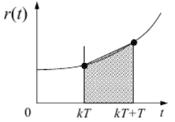
When writing this abstract, the master's work has not yet been completed. Final completion: June 2021. The full text of the work and materials on the topic can be obtained from the author or his supervisor after the specified date.
Contents
- Introduction
- 1. Classification of systems of recognition
- 2. real-time Recognition
- 3. Equipment requirements for the recognition system
- 4. Preparation of a data set
- 5. Neural Network Cloud Learning
- 6. Laboratory Plant Design Description
- 7. RS-485 and RTU ModBus Protocol
- 7.1 Description RS-485
- 7.2 Description ModBus RTU
- 7.3 Implementation on microcontroller stm32
- 8. Synthesis of a discrete control system
- 8.1 Synthesis of a single–circuit control system with discrete PI-RS
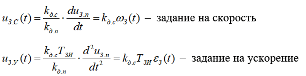
- 8.2 PD synthesis of tracking system position control
- 8.3 Discrete setter of situation
- Conclusion
- References
Introduction
In recent years, more enterprises have moved from manual sorting to a more efficient automated solution, sorting systems.
The use of conveyors for sorting allows you to significantly increase both the profitability and productivity of many cargo operations and are an integral part of many distribution centers and industries. Automatic cargo sorting, used in the process of conveyor movement, significantly reduces the cost of manual labor for their further processing: packaging on pallets, for further transportation, etc. And the use of machine vision, namely, the object recognition system, creates effective competition for systems based only on sensors. As in such systems several characteristics of an object are analyzed at once: color, form, sizes, texture, drawing, pattern, etc. Also, such systems are easily supplemented and improved by the same sensors to increase efficiency.
1. Classification of systems of recognition
There are several basic object detection algorithms that can be divided into two groups:
-
Algorithms based on classification.
They are implemented in two stages. First, the algorithm selects areas of interest in the image. Then, these regions are classified using convolutional neural networks. This solution can be slow, because we need to run forecasts for each selected region. A well-known example of this type of algorithm is the region-based convolutional neural network (RCNN) and its relatives Fast-RCNN, Faster-RCNN and the latest addition to the family: Mask-RCNN. Or RetinaNet.
R-CNN (Regions with Convolution Neural Networks features): R-CNN, Fast R-CNN, Faster R-CNN, Mask R-CNN. To detect an object in an image using the Region Proposal Network (RPN) mechanism, limited regions (bounding boxes) are allocated. Initially, a slower Selective Search mechanism was used instead of RPN. The allocated restricted regions are then fed to the input of the conventional neural network for classification. In the R-CNN architecture, there are clear cycles of
for
search by limited regions, up to 2000 runs through the internal AlexNet network. Due to explicitfor
cycles, the speed of image processing slows down. The number of explicit cycles, runs through the internal neural network, decreases with each new version of the architecture, and dozens of other changes are made to increase speed and to replace the task of detecting objects with segmentation of objects in Mask R-CNN. -
Regression-based algorithms.
Instead of selecting interesting parts of the image, they define classes in one run of the algorithm. Two of the most famous examples from this group are the algorithms of the YOLO (You Only Look Once) and SSD (Single Shot Multibox Detector) family. They are usually used to detect objects in real time, since, as a rule, they sacrifice accuracy for a significant increase in speed. YOLO is the first neural network to recognize real-time objects on mobile devices. A distinctive feature: distinguishing objects in one run (it is enough to look once). That is, in the YOLO architecture there are no explicit
for
cycles, which is why the network works quickly. For example, such an analogy: in NumPy, during operations with matrices, there are also no explicitfor
cycles, which are NumPy implemented at lower levels of the architecture through the programming language. YOLO uses a grid from predefined windows. Use the window overlap factor (IoU, Intersection over Union) to prevent the same object from being defined multiple times. This architecture works in a wide range and has high robustness: the model can be trained in photographs, but at the same time work well in painted paintings.SSD –
khaki
of YOLO architecture (for example, non-maximum suppression) are used and new ones are added to make the neural network faster and more accurate. A distinctive feature: distinguishing objects in one run using a given grid of windows (default box) on the pyramid of images. The image pyramid is encoded in convolutional tensors during successive convolution and pooling operations (during the max-pooling operation, the spatial dimension decreases). This defines both large and small objects in a single network run.
2. real-time Recognition
In the case of real-time recognition, regression-based algorithms are used, since instead of choosing interesting parts of the image, they determine classes in one run of the algorithm, which significantly increases the speed.
When the YOLOv1 was released in 2016, the accuracy-speed indicators were comparable to the SSD indicators, in addition, the YOLOv1 is more easy to apply. YOLO is actively supported and improved, and with each new generation it becomes faster, more precisely.
The improved YOLOv2 exceeded the SSD speed, and the special configuration with the abbreviation -tiny developed for applications in mobile devices significantly increased the speed of work, but sacrificed accuracy. -tiny also got its continuation in subsequent generations.
YOLOv3 stepped even further increasing its performance in both accuracy and speed. Undoubtedly, the latest generation of YOLOv4 is the fastest and most accurate object recognition system among its competitors.
The obvious choice for real-time recognition is YOLO. All because YOLO specifically designed for use in mobile devices does not have explicit for
cycles, and is also completely written in C, which is one of the successful solutions for a high-speed recognition system.
As this regression-based algorithm has already been said, instead of selecting interesting parts of the image and classifying them, it determines classes by scanning the entire image in one run of the algorithm. The whole image scanning process begins with a predetermined n * n pixel window, which produces a logical result that is true if the specified object is present in the scanned portion of the image, and false if it is not. After scanning the entire image, the algorithm increases the window size that is used to re-scan the image. Methods based on deformable part models for object detection (DPM) use this technique, which is called a sliding window. The YOLO model was developed for an open source neural network based on DarkNet. But one DarkNet implementation is not limited, YOLO can be implemented on Keras and on the same Tensorflow. But DarkNet fully meets the requirements, since it is also completely written in C, which means that speed within the framework of real iron is guaranteed.
Figure 1 – Sliding window (animation: 98 frames, 6 cycles, 277 KB)
3. Equipment requirements for the recognition system
Tasks of this kind require appropriate equipment, and in the case of automation of the production line, it becomes a question of profitability and price-speed ratio of such a system. Therefore, solutions aimed at using the cheapest possible equipment will be considered. The presented approach is suitable for almost any equipment, whether it is a laptop with a built-in graphics core, or Raspberry-pi. Since our implementation uses CPU instead of the recommended and fast GPU. This will negatively affect the speed of work, literally tens of times. But it will provide an opportunity to study the features and implement the system for literally everyone.
It is important to clarify the question of testing and working on this equipment, training and tuning on such machines will be very difficult, since such convolutional neural networks require sufficiently powerful computing capabilities that only the GPU can provide.
The rule for selecting a GPU for machine learning is:
- Capacity metrics, working with RNN
- FLOPS key figures, work with rollup
- Use tensor cores if you can afford.
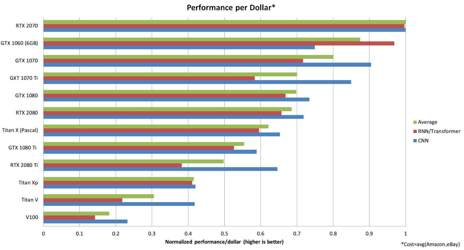
Figure 2 – Performance Statistics
This data shows that RTX 2070 is more cost effective than RTX 2080 or RTX 2080Ti. Why is that? The ability to perform 16-bit calculations with Tensor Cores is much more valuable than simply having a large number of tensor cores. With RTX 2070 you get these features at the most optimal price. New RTX 30xx series cards are not included in this comparison because data on them is not enough.
Preparation of a data set
Before you begin training, you must prepare a sufficiently large data set of a specific format. To train the network for certain objects, you need to create a data set in which photos will be stored that contain the necessary objects in the .jpg format and their corresponding .txt files in which the coordinates of the areas on which the objects of interest are depicted will be stored. To do this, we use an open git repository LabelImg, this program, specially written to solve this kind of problem.
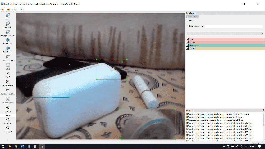
Figure 3 – Operating window of the program LabelImg
The .txt file stores data for each object in a new row in a given order:
[object-class] [x] [y] [width] [height], где:
[object-class] is an integer number of objects to recognize from 0 to (N-1).
[x] [y] is the center of the rectangle.
[width] [height] – floating point values relative to the width and height of the image, ranging from 0.0 to 1.0.
Example of this file:
2 0.703750 0.208437 0.430833 0.353125
3 0.276667 0.330937 0.395000 0.291875
0 0.572917 0.513437 0.222500 0.096875
1 0.479583 0.687187 0.165833 0.233125
I recommend taking as many photos of objects as possible from different angles, with different lighting, different background, the presence of similar things in the background will also be positively reflected in order to more clearly show the networks details and distinctive features of given objects.
I also recommend making mirror copies horizontally or vertically and classifying them. The neural network recognizes these images as new, which will positively affect recognition in different planes. Knowing how the label file is formed, and after a little understanding of several python libraries, you can write a simple program that rejects the image along the X and Y axes and, according to the necessary rules, creates labels for them in a separate .txt file. In this part of the work, everyone is expelled in their own way, I will not describe my program, not on a topic.
At the exit, we will have so much-needed photos of objects and their corresponding label files, and with the use of recalculation, their number can be safely multiplied by 3.
The database created must be divided into data that will be directly trained and data for validation.
5. Neural Network Cloud Learning
The absence of recommended but expensive equipment does not impede our goal, but only creates certain conditions. Based on this, you can use cloud resources that provide your computing capabilities to train your network. My choice fell on Google Colab.
Google Colab is a free cloud service based on Jupyter Notebook with Python 2-3 support, from the box. Google Colab provides everything you need for machine learning right in the browser, gives you free access to incredibly fast GPUs and TPUs. But unfortunately, it imposes some restrictions, such as a time limit of 12 hours after which you will be disconnected from the virtual machine, and the ability to use only one graphics processor provided to you from among the currently available ones. These GPUs have minimum requirements that meet training requirements, but still have different characteristics.
Since the implementation is carried out as part of the use of low-power equipment, we use DarkNet, and the weighting file darknet53.conv.74 . Before you begin training, you need to make sure that your Google Colab notebook uses a GPU, you also need to recompile Makefile based on the capacity used, create your own configuration yolov3_training.cfg preferably based on the original yolov3.cfg, or yolov4.cfg if a newer version is used.
Last is to create a .names file that specifies the classes, their number, and their location paths. Since we use a cloud resource, their location will be locally virtual machine.
Training will take a very long time, and most often it will take much more than 12 hours of Google Colab dedicated to real accurate indicators, so I recommend re-saving the .cfg weight file every 100 eras to the same cloud resource Google Drive. This will facilitate the process many times, thanks to this, when the emission expires after 12 hours, and most often even earlier you will not lose data and you will be able to continue your training based on this scale file. But keep in mind that Google Drive has a limit of 15Gb so I recommend that you clear out-of-date weight files.
6. Laboratory Plant Design Description
The object of automation is a sorting conveyor with a position guide. The position of the track, as well as the entire conveyor movement algorithm, is controlled using the stm32f407vzt6 controller. The controller collects information from the sensors and the recognition system, based on this information, generates signals that control the drives of the conveyor.
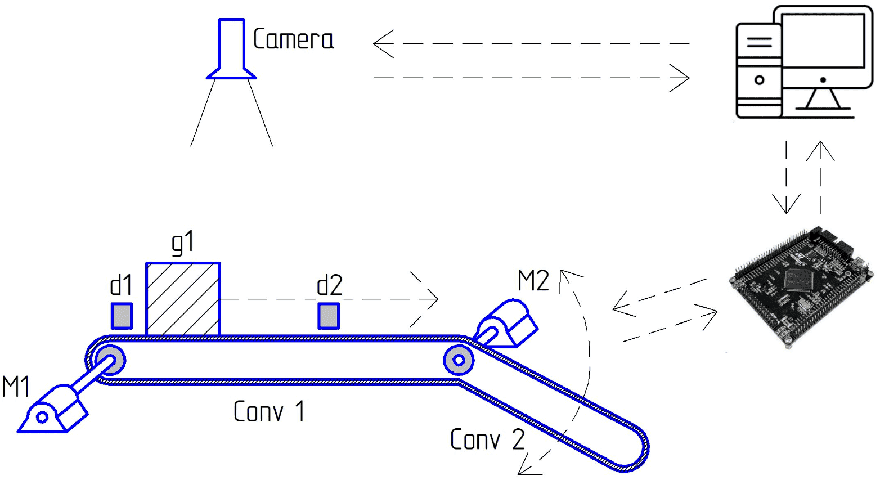
Figure 4 – Simplified design of laboratory plant
Sensor set used in the system:
Optical sensors, or pressure sensors, are used to signal the arrival and departure of the sorting object.
The same sensors can be used to pre-check an object, which will increase the accuracy of sorting.
You must use a Hall sensor or encoder to control the drives.
It is important to clarify if this design will be deliberately used in production, then the connection between the recognition system and the microcontroller is implemented by Serial Port or SPI a very unstable solution. That is why it is necessary to make the transition from Serial Port (USART RS-232) to industrial standard RS-485 and protocol ModBus.
7. RS-485 and ModBus RTU protocol
7.1 Description RS-485
The RS-485 interface (another name is EIA/TIA-485) is one of the most common standards for physical layer communication. The physical layer is a communication channel and a method of signal transmission (layer 1 of the open OSI interconnection model).
СThe network built on the RS-485 interface is a transceiver connected by twisted pair – two twisted wires. The RS-485 interface is based on the principle of differential (balance) data transmission. Its essence is the transmission of one signal over two wires. And one wire (conditionally A) carries the original signal, while the other (conditionally B) carries its inverse copy. In other words, if one wire has 1
, then the other has 0
and vice versa. Thus, there is always a potential difference between two twisted pair wires: with 1
it is positive, with 0
it is negative.
Figure 5 – United States using twisted pair technology
It is this potential difference that the signal is transmitted. This transmission method provides high resistance to in-phase interference. Common phase interference is referred to as interference acting on both wires of a line in the same way. For example, an electromagnetic wave passing through a section of a communication line carries potential in both wires. If the signal is transmitted by a potential in one wire relative to the common one, as in RS-232, then the lead on that wire can distort the signal relatively well absorbing the common lead (ground
). In addition, on the resistance of a long common wire, the difference in potential between the earths will drop – an additional source of distortion. And with differential transmission, no distortion will occur. In fact, if two wires run close to each other and are twisted, the lead on both wires is the same. The potential in both equally loaded wires changes equally, while the informative potential difference remains unchanged.
Hardware implementation of the interface – transceiver chips with differential inputs/outputs (to the line) and digital ports (to UART controller ports). There are two versions of this interface: RS-422 and RS-485.
RS-422 – full duplex interface. Reception and transmission are carried out over two separate pairs of wires. There can only be one transmitter on each wire pair.
RS-485 – half duplex interface. Reception and transmission are carried out on the same pair of wires, separated by time. There can be many transmitters in the network, as they can be switched off in reception mode.
Figure 6 – RS-422 and RS-485
D (driver) – transmitter;
.R (receiver) – receiver;
.DI (driver input) – digital transmitter input;
RO (receiver output) – digital receiver output;
DE (driver enable) – authorization of transmitter operation;
RE (receiver enable) – authorization of the receiver;
A – direct differential input/output;
.B – inverse differential input/output;
.Y – direct differential output (RS-422);
Z – inverse differential output (RS-422).
I will stop for more details on the RS-485 transceiver. The digital output of the receiver (RO) is connected to the UART receiver port (RX). The digital transmitter input (DI) is connected to the UART transmitter port (TX). Since on the differential side the receiver and the transmitter are connected, the transmitter must be switched off during reception and the receiver during transmission. The control inputs for this are the receiver resolution (RE) and the transmitter resolution (DE). Since the RE input is inverse, it can be connected to DE and the receiver and transmitter can be switched with one signal from any controller port. At level 0
– work on reception, at level 1
– on transmission.
Figure 7 – RS-485 connection
The receiver receives a potential difference (UAB) at the differential inputs (AB) and converts it into a digital signal at the RO output. The sensitivity of the receiver may vary, but the guaranteed threshold range for signal recognition is written by the manufacturers of transceiver chips in the documentation. Usually these thresholds are ± 200 mV. That is, when UAB >+ 200 mV – the receiver defines 1
, when UAB <= 200 mV – the receiver defines 0
. If the potential difference in the line is so small that it does not exceed the thresholds – correct recognition of the signal is not guaranteed. In addition, there may be non-phase interferences in the line that will distort such a weak signal.
All devices are connected to one twisted pair in the same way: direct outputs (A) to one wire, inverse outputs (B) to another wire.
The input resistance of the receiver on the line side (RAB) is usually 12 KOhm. As the transmitter power is not unlimited, this creates a limit on the number of receivers connected to the line. According to the RS-485 specification with matching resistors, the transmitter can drive up to 32 receivers. However, there are a number of chips with a higher input resistance, which allows significantly more than 32 devices to be connected to the line.
The maximum communication speed on the RS-485 specification can reach 10 Mbps. The maximum distance is 1200 m. If it is necessary to organise communication over a distance of more than 1,200 m or to connect more devices than the load capacity of the transmitter permits, special repeaters (repeaters) are used.
7.2 Description ModBus RTU
The Modbus protocol assumes that only one master (controller) and up to 247 slaves (Bus Terminals) can be connected to an industrial network. The exchange of data is always initiated by the master. The slaves never start the data transfer until they have received a request from the master. The slaves cannot exchange data with each other either. Therefore, only one exchange act can take place in the Modbus network at any given time.
Addresses 1 to 247 are Modbus addresses on the network and 248 to 255 are reserved. The master device must not have an address and there must not be two devices with the same addresses in the network.
The master device can send requests to all devices simultaneously (broadcast mode
) or to only one device. Address 0
is reserved for the broadcast mode (if this address is used in a command, it is accepted by all devices in the network).
In the Modbus RTU protocol, the message starts to be perceived as new after a bus pause (silence) of at least 3.5 characters (14 bits), i.e. the value of the pause in seconds depends on the transmission speed.
The format of the frame is shown in the picture:
Figure 8 – Modbus RTU protocol frame format
PDU – Protocol Data Unit
– Protocol Data Element
;
ADU – Application Data Unit
– application data element
Address field always contains only the address of the slave device, even in response to a command sent by the master. This means that the master knows which module the response has come from.
.The Function code
field tells the module what action to perform.
The Data
field may contain any number of bytes. It may contain information about parameters used in controller queries or module responses.
The checksum
field contains a CRC checksum of 2 bytes in length.
In the RTU mode, the data is transmitted with lower bits forward.
Figure 9 – Bit sequence in RTU mode
Parity bits in RTU mode are set to 1 if the number of binary units in the byte is odd, and to 0 if it is even. This parity is called even parity, and the control method is called parity control.
The even number of binary units in byte parity bits may be equal to 1. In this case the parity is said to be odd parity.
The parity check may not exist at all. In this case, a second stop bit must be used instead of a parity bit. To ensure maximum compatibility with other products, it is recommended that the option of replacing the parity bit with a second stop bit be used.
Some devices can perceive any of the options: even, odd parity or no parity.
Modbus RTU messages are transmitted as frames, for each of which the beginning and end are known. The sign of the start of the frame is a pause (silence) of at least 3.5 hex characters (14 bits). The frame must be transmitted continuously. If a pause of more than 1.5 hex characters (6 bits) is detected in the transmission, the frame is considered to contain an error and must be rejected by the receiving module. These pause values must be strictly adhered to at speeds below 19200 bps, but at higher speeds, fixed pause values of 1.75 ms and 750 µs are recommended, respectively.
In RTU mode there are two levels of error control in the message:
.- parity control for each byte (optional);
- control the entire frame using the CRC method.
CRC method is used independently of parity checks. The CRC value is set in the master before the transmission. When a message is received, the CRC for the entire message is calculated and compared with the value specified in the CRC frame field. If both values are the same, the message is considered to contain no error.
Starts, stop bits and parity bits are not involved in the CRC calculation.
7.3 Implementation on microcontroller stm32
I took the port as a basis FreeModbus from a Chinese friend of Armink.
It will take a lot of time to describe everything, and I will explain briefly what and where I made the corrections:
File mb.c\mb.h and the initialisation function, in file mbport.h, new announcements have appeared which are used in mbrtu.c in the corrected code section of the function xMBRTUTransmitFSM, porttimer.c, now it is possible to completely abstract from a specific timer, portevent_m.c had to be adapted to work without RTOS. The port porttimer.c file, with the addition of macros for the RTS line, the initialisation, flow switching, receiving and sending functions (and a new one added – xMBPortSerialPutBytes) have also been simplified. And a bunch of other little things.
All in all, this was done for the purpose of unification: Organise the possibility of using HAL with minimal changes in portserial and porttimer files. Remove peripheral initialization from the portserial and porttimer files, since when using HAL it already occurs before FreeModbus initialization is called. Add the sending of the package to portserial as a whole, not as a pooling of one byte each. Add byte acceptance by DMA or interrupt, not byte pulling one byte at a time.
8. Synthesis of a discrete control system
8.1 Synthesis of a single-circuit control system with discrete PI-RS
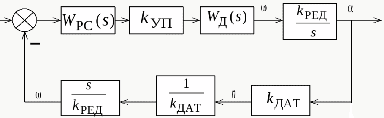
Figure 10 – Generalized cattle structure diagram
PF an open RS system:

Take the constant anchor chain and thyristor converter as insignificant, then:
![]()
Then the RKS for Modular Optimum:
As a result, PF-RS has a look:
![]()
Proportional coefficient kp and integral ki have a form:
![]()
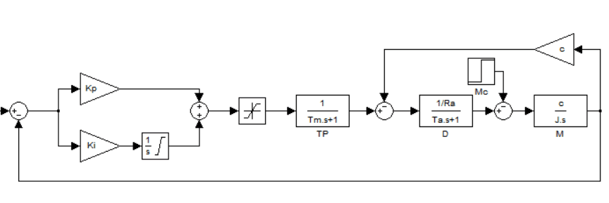
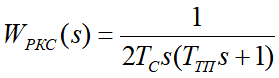
Figure 11 – Complete single-circuit ATS speed model in MATLAB Simulink package
The given regulator must be brought to a discrete form as it describes continuous transformations.
There are several basic substitution methods for sampling continuous objects:
Euler's method
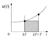
Inverse difference method
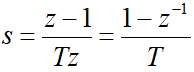
Tastin method
In using the Tastin method, or as it is also called the trapezoidal PI method, the discrete PI regulator will look like:
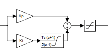
Figure 12 – Discrete PI-RS
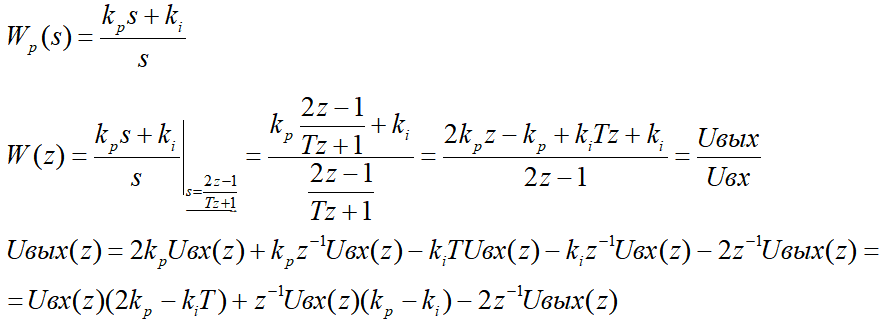
Plot the expression into simple multipliers and use the z-conversion rules to move from the operator form to the lattice function view:
.![]()
8.2 Synthesis of the PD regulation of the tracking system
.The main controllable coordinate in such systems is the position (movement) of the executive body (EO) of the working machine. Position sensors (DPs) are two types of devices installed on the motor shaft or the IE – analogue or discrete.
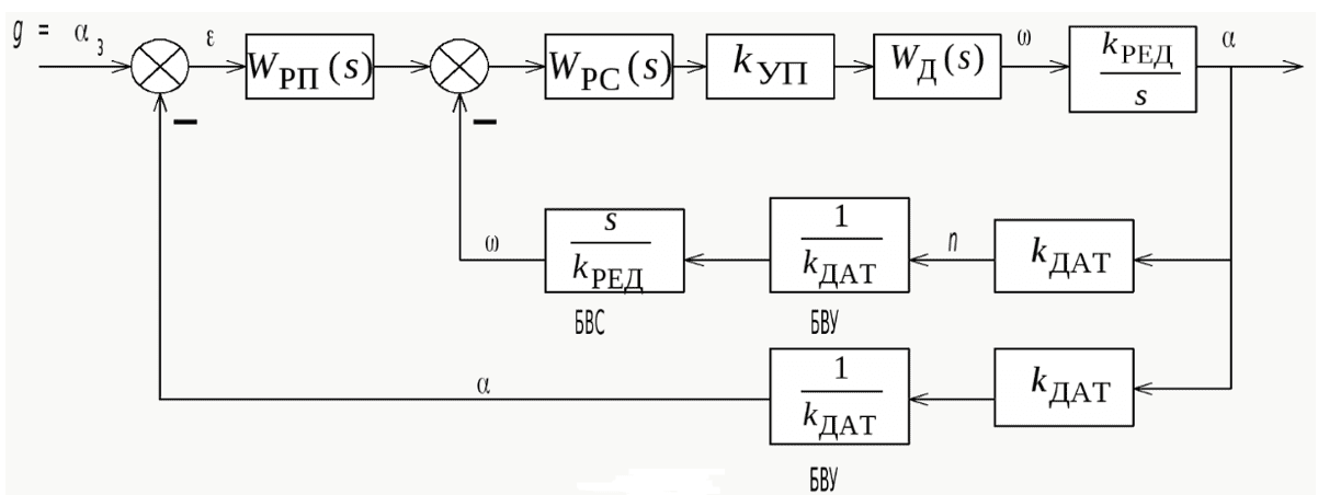
Figure 13 – Generalized structural diagram of the position management system (tracking systems)
The construction of a position control system consists in the organisation of a control loop external to the speed loop, closed on the movement of the engine shaft or the IE. As a speed control system (SPC), any of the possible systems can be used in principle, in our case we use the system described above to control the conveyor belt. The output of the position controller (PSD) is limited to a level corresponding to the maximum permissible speed (taking into account the reserve for over-regulation in the dynamics, which should be selected taking into account the static load, which is usually 1...5%).
Position control systems based on single-zone CPCs are the most common, so the maximum allowed speed is the value of the ideal idle speed, taking into account the reserve for over-regulation in dynamics.
Let's assume that the transitional function of the aperiodic link is initially different from that of the integrating link in the initial time interval. On this basis, the structural diagram of the control object can be presented as follows:
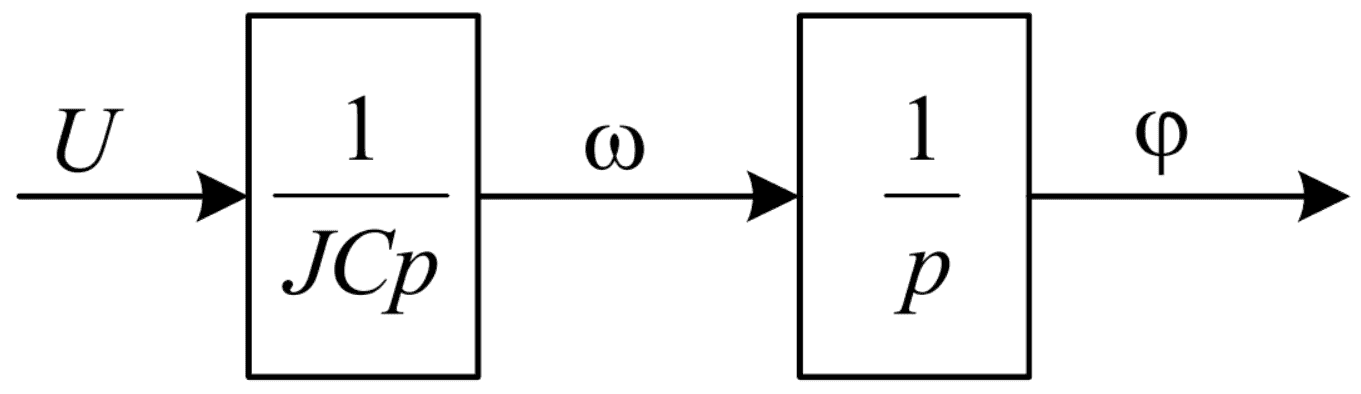
Figure 14 – Control object
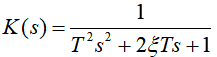
Using the PD, the position controller can be considered as a reference model of a control object the oscillating link with a time constant T that meets the requirements for the speed of the actuator and a damping factor.
Then we will get a structural diagram with the assumptions accepted:
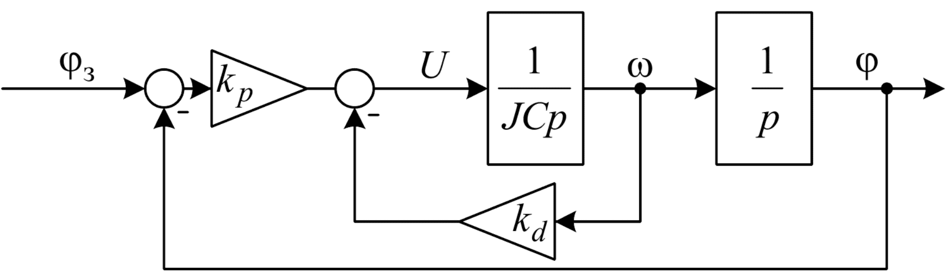
Figure 15 – Positioning Tracking System with AP Controller
The PF of such a system has the appearance:
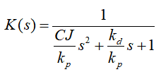
Based on the requirement of matching the numeric values of the transfer function coefficients, we will obtain the following values of the PD regulator coefficients:
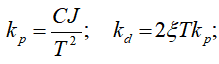
Beginning from the fact that the PD regulator is actually set by coefficients without increasing the order of the system, this regulator does not need any sampling. In this case, the same coefficients from the continuous system will be used in the discrete system.
.8.3 Discrete setter of situation
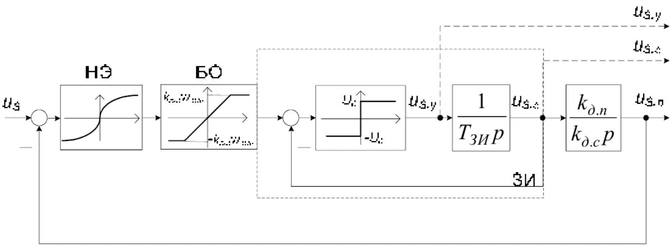
Figure 16 – Structural diagram of the setter of situation
Taking into account that the SI parameters:
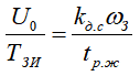
The SS output signal:
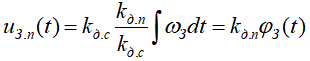
This allows you to set the ideal chart of change of the adjustable coordinate (position) in a non-inertial slave system of position control.
This eliminates the need to use ZI at the input of the speed control loop.
An important advantage of WP application is the possibility of obtaining derivatives from the target effect without the use of differentiation operation:
With the help of these signals the principle of combined control is implemented, which allows to provide a sufficiently high speed of the position control loop (PLC). This principle is very important for position control (as the equivalent inertia of the position control system is already quite significant).
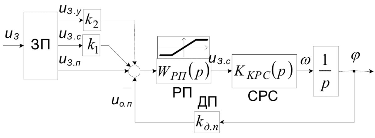
Figure 17 – PSA structural scheme with SS
In this case, all regulators of the system operate in a linear mode, and the speed and acceleration limitation is carried out due to the special generation of a reference signal at the PFC:
![]()
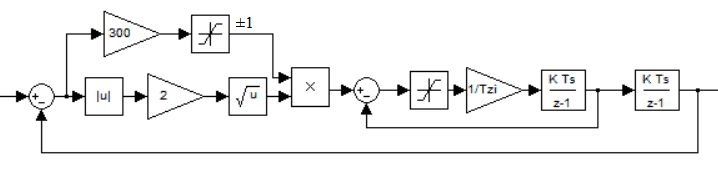
Figure 18 – The structural diagram of discrete SS
Conclusion
In this essay, general descriptions of the main components of the thesis were presented. There were no methods of matching the equipment and describing the programs of microcontrollers due to the cumbersomeness and lack of desire. Briefly, all signals were coordinated by levels. For example, PWM signals controlling the driver motors were converted from the logical unit of the microcontroller stm32 which is 3.3 volts to the logical unit of the driver 5 volts. Thanks to MOSFET N-channel transistors with the lowest possible gate voltage (IRL3502 or BSS138).
It is also planned to introduce a separate control panel connected via UART to the main controller. The remote will be a separate microcontroller on which it is planned to connect SPI TFT ili9341 display and accordingly a simple keyboard, possibly a sensor. However, it is not yet clear whether this will come to fruition.
When writing this essay, the master's work is not yet complete. Final completion: June 2021. Full text of the work and materials on the topic can be obtained from the author or his manager after the specified date.
References
- Основные типы сортировочных конвейеров В. Голышев [Electronic resource]. Access mode: https://sitmag.ru/article/10018-osnovnye-tipy-sortirovochnyh-konveyerov(date of circulation 28.11.2020).
- YOLO Real Time Object Detection on CPU [Electronic resource]. Access mode: https://pysource.com/2019/07/08/yolo-real-time-detection-on-cpu/(date of circulation 28.11.2020).
- YOLO: real-time Object Detection [Electronic resource]. Access mode: https://github.com/tzutalin/labelImg(date of circulation 28.11.2020).
- RM0090 Reference manual STM32F405/415, STM32F407/417, STM32F427/437 and STM32F429/439 advanced Arm®–based 32-bit MCUs / www.st.com, February 2019. – 1749 с.
- DoclD022152 Datasheet STM32F405xx STM32F407xx ARM Cortex-M4 32b MCU+FPU, 210DMIPS, up to 1MB Flash/192+4KB RAM, USB OTG HS/FS, Ethernet, 17 TIMs, 3 ADCs, 15 comm. interfaces & camera / www.st.com, September. – 202 с.
- FreeModbus datasheet [Electronic resource]. Access mode: https://www.embedded-solutions.at/files/freemodbus-v1.6-apidoc/, (date of circulation 28.11.2020).
- Инструкция по работе с TensorFlow Object Detection API [Electronic resource]. Access mode: https://habr.com/ru/company/nix/blog/422353/, (date of circulation 28.11.2020).