
Abstract
Содержание
- Introduction
- 1 Neuron and neural network
- 1.1 Biological neuron
- 1.2 Mathematical model of neuron
- 1.3 Basic types of neural network architectures
- 1.4 Basic concepts of neural networks
- 1.5 Convolutional neural networks
- 2. Neural network for color recognition in the MATLAB software package
- Conclusions
- List of sources
Introduction
Currently, the industry is widely used vision systems, which help to obtain visual information about the technological process. This information often carries important information about the current state of the technological process. One of the ways to obtain and process such information at present is the use of artificial neural networks. Modern neural networks make it possible to classify objects with great accuracy, divided into thousands of different classes, do an excellent job with image recognition, for example, such systems are used in security systems for face recognition or in fingerprint scanners. With the help of neural networks in enterprises, it is possible to predict equipment failure and promptly carry out repairs, which will reduce downtime, since in large industrial enterprises even the slightest downtime can lead to large financial losses. In medicine, artificial neural networks help predict the development of diseases, as well as identify existing diseases in the early stages, when doctors find it difficult to determine.
1 Neuron and neural network
1.1 Biological neuron
A neural network is a sequence of neurons connected by synapses. The structure of the neural network came to the programming world straight from biology. Thanks to this structure, the machine acquires the ability to analyze and even memorize various information. Neural networks are used for classification problems, regression, information compression, recovery of lost information, etc.
Schematically, a biological neuron looks like it is shown in Fig. 1.1.
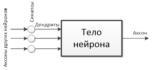
Fig 1.1 - Schematic view of a biological neuron.
The most important parts of a neuron are: the body of the neuron, axons, dendrites and synapses. The body of a neuron stores information from other neurons, processes it, and transmits it to other neurons. Dendrites are neuron processes that receive information from other neurons. Axon is a process of a neuron, with the help of which information processed by the body of a neuron is transmitted to other neurons. The synapse is the junction of the axon of one neuron with the dendrite of another neuron, it determines how important this connection is for the neuron receiving information.
1.2 Математическая модель нейрона
Математическая модель нейрона представлена на рис.1.2.
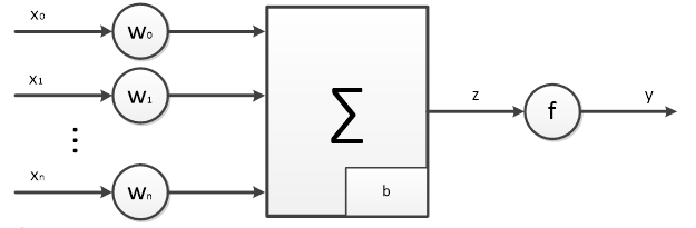
Fig. 1.2 - Mathematical model of a neuron
In the mathematical model, the inputs are x0-xn, which can be any finite number. The weights w0-wn act as a synaptic connection, which determine how informative a particular input is for a given neuron. An adder is presented as the body of a neuron, which adds up all inputs to it, and also takes into account the deviation b. The signal from the output of the adder is transmitted to a certain function, which is called the activation function and determines whether at this moment in time the output y will be in an excited state.
The mathematical model of a neuron is described by the following expression:
The w0-wn and b parameters are configurable and change as the neural network is trained. It is in the selection of the optimal values of these parameters that the learning process of the neural network consists. F(z) is the activation function (transfer function) of the neuron, which, based on the input signals, determines whether the output of the neuron is active at the moment.
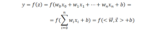
The simplest activation function is the threshold function, which looks like the one shown in Fig. 1.3.
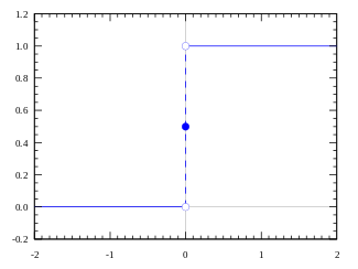
Fig 1.3 - Threshold function of neuron activation
Also, in practice, they are often used:
- linear activation function:
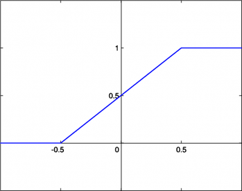
Fig 1.4 – Linear neuron activation function
- sigmoidal activation function:
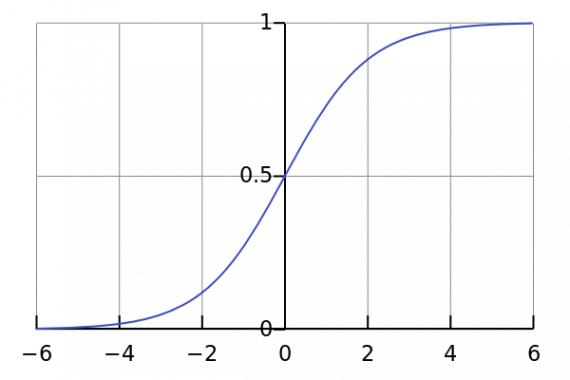
Fig 1.5 – Sigmoidal neuron activation function
- hyperbolic tangent:
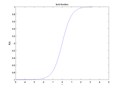
Fig 1.6 – Activation function - hyperbolic tangent
1.3 Basic types of neural network architectures
When designing a neural network, an important point is the choice of its architecture. The choice of architecture affects the learning ability of the network, choosing different architectures of the neural network can both learn at different speeds and with different accuracy. Thus, if the wrong network architecture is chosen, the network will not be able to correctly learn the task at hand.
In general, a network is a set of neurons interconnected in a certain way.
The main types of neural network architectures are:
- Direct distribution networks. In such NS, the signal goes from the input only towards the output of the NS. Such neural networks can have either one layer of neurons or several layers at once. An example of a single-layer feedforward neural network is shown in Fig. 1.7.
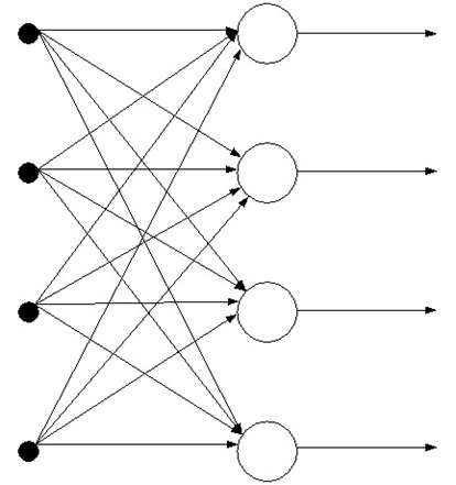
Fig 1.7 - Single layer feedforward neural network.
An example of a multi-layer feedforward neural network is shown in Fig. 1.8.
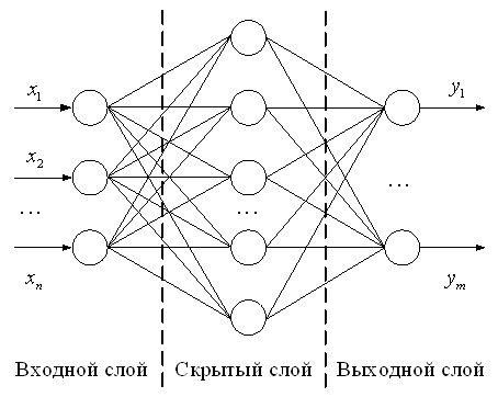
Fig. 1.8 – Multilayer feedforward neural network.
- Feedback networks. In such neural networks, information from subsequent layers is transferred to the previous ones. Feedbacks can cover both individual neurons and layers of the neural network, as well as the entire network as a whole. The introduction of feedbacks can both positively affect the operation of the network, expanding its functionality, and negatively, affecting its stability. An example of a neural network with feedback is shown in Fig 1.9.
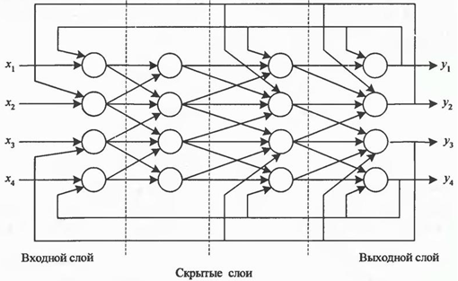
Fig 1.9 – Feedback neural network
In practice, when applying neural networks with feedback, Hopfield networks are most often used, the architecture of such a network is shown in Fig 1.10.
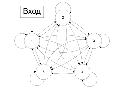
Fig. 1.10 – Hopfield network
- Regular or competing networks. In such neural networks, neurons are located at the main nodes of some regularization lattice. Each neuron of such a neural network is connected in a certain way with its neighbors. The neighborhood of neurons is determined by the type of regularization grid used. An example of a competing neural network is shown in Fig. 1.11.
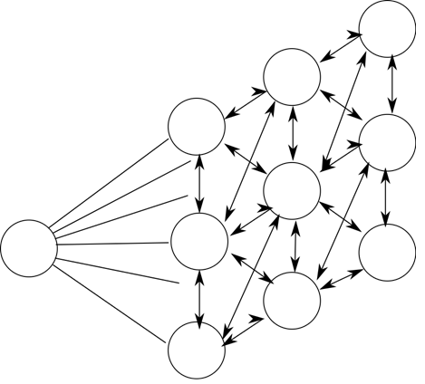
Fig 1.11 – Kohonen's Competing Neural Network
Cohenen's competing neural networks are self-learning and do not require a labeled training set for training, which is called unsupervised learning.
In known neural networks, several types of neuron structures can be distinguished: homogeneous and heterogeneous. Homogeneous NN consist of neurons of the same type with the same activation function.
Also NN are divided into binary and analog. In binary NS, only binary signals are used, and in analogue signals, arbitrary signals. Neural networks are classified into synchronous and asynchronous. In the first class, only one neuron changes its state at a time. In the second, entire groups of neurons (for example, the entire layer) can change their state.
1.4 Basic concepts of neural networks
With the help of a single neuron, objects can be classified linearly on the classifying surface. An example of such a surface is shown in Fig. 1.12.
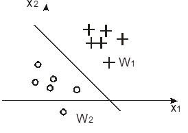
Fig 1.12 - Two linearly separable classes
However, the dividing surface of the network is not linear. With the help of a two-layer neural network, which on the first layer has an activation function - a sigmoid, and on the second layer - a linear activation function, it is possible to approximate any nonlinear dependence with a finite number of points on the dividing plane. An example of a nonlinear dependence is shown in Fig. 1.13.
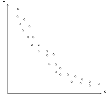
Fig 1.13 - Non-linear dependency
To build a neural network, you need to decide on:
- NN architecture;
- loss function;
- optimization method;
- metrics.
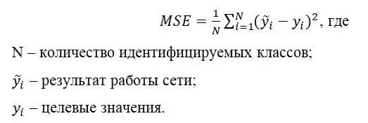
The loss function helps determine the accuracy of the neural network. The simplest loss function is the root mean square error, which is calculated using the formula:
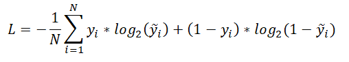
The following loss functions are also the most used:
- Cross entropy, which is calculated by the formula:
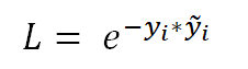
- Exponential loss function:
For each specific task, you must reasonably choose your own loss function.
The neural network optimization method determines how it is necessary to change the weights of neurons in order to solve the problem. The most popular optimization method for neural networks is the gradient descent method and its modifications, such as stochastic gradient descent with momentum (SGDM), etc. The optimization method should be chosen so that the loss function tends to the global minimum of its function. For each specific neural network, it is necessary to select its own optimal optimization method, and it is difficult to predict in advance which method will show itself better in this or that case. Graphically, the gradient descent method is shown in Fig. 1.14.
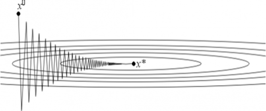
Fig 1.14 - Graphical representation of the gradient descent method
X0 is the result of the operation of the first iteration of the NN, and X * is the local minimum of the loss function, to which it is necessary to strive. The convergence rate is influenced by the step of the gradient descent, which is selected for each NN individually, however, if the wrong step is chosen, the results of the NN operation may not fall into the minimum point of the loss function.
Metrics mean a way to track the results of the neural network at each iteration. Most often, the percentage of deviation of the results of the neural network from the values that was expected to be seen at its output is calculated.
1.5 Convolutional neural networks
In practice, convolutional neural networks are used to work with data such as images. Such networks with great accuracy solved the problem of recognizing handwritten numbers, which are contained in the MNIST library. Also, many convolutional neural network architectures appeared that were able to solve the ImageNet Challenge, which is to train neural networks to recognize 1000 different classes on a dataset of 150,000 examples. The essence of convolutional neural networks is to filter out information that is not useful for the neural network using convolution (filtering), as well as to recognize different classes regardless of their location and size in the image.
Since the image is a matrix of pixels, a certain matrix is applied to the image, called a mask (filter), and a new matrix is obtained on its basis. Typically, many such filters are applied in order to understand what data is in the original image using various masks. Next, a pooling layer is applied, this layer is used to discard unnecessary information. The pooling layer finds the maximum, minimum, or average value of matrix elements in a specific area. After that, the layers are repeated until the output is represented as a column vector, and then this data is transferred to a fully connected layer, which has the same number of neurons as the number of classes that need to be identified in the images. Then, using the SoftMax layer, the probabilities that the image contains a particular class are given to the output of the neural network.
The first convolutional neural network to make a breakthrough in recognition was the LeNet network, presented in 1998 and the architecture of this network is shown in Fig. 1.15.
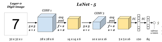
Fig 1.15 - Architecture of the LeNet convolutional neural network
After that, convolutional neural networks began to improve in such a way as to show the best results on the MNIST training dataset. There were such architectures as:
- AlexNet (2012), shown in Fig. 1.16;
- VGG (2014), shown in Fig. 1.17;
- GoogLeNet (2015), a modified version of Google's LeNet architecture, is shown in Fig. 1.18.
- ResNet, представлена на рис. 1.19.
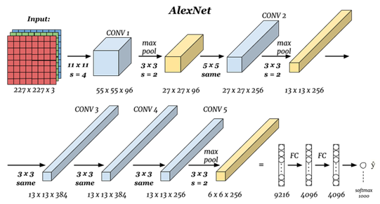
Fig 1.16 - AlexNet convolutional neural network architecture
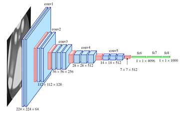
Fig 1.17 - VGG convolutional neural network architecture
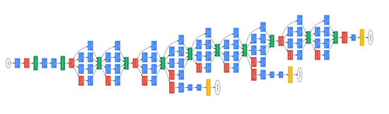
Fig 1.18 - GoogLeNet convolutional neural network architecture
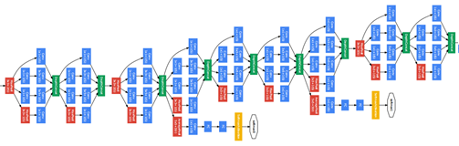
Fig 1.19 - ResNet convolutional neural network architecture
2. Neural network for color recognition in the MATLAB software package
To create a neural network, which in the future needs to be trained for color recognition, it was decided to use the supervised learning method. To do this, you must have a set of data on which training will take place - a training sample. A training sample for a given task can be generated using a script, which was done:
from PIL import Image
for i in range(240,256):
for j in range(230,256):
for k in range(0,40):
img = Image.new("RGB", (140,140), (i,j,k))
img.save("D:\\colors\\yellow\\" + str(i) + "_" + str(j) + "_" + str(k) + ".jpg","JPEG")
The script is written in the Python programming language and performs the following actions: for a certain range of colors in RGB format, it generates a work plane of 140 x 140 pixels and fills it with pixels of the current color, then the result is saved in a specific folder with a name corresponding to this color. Then, using nested loops, the color changes and the actions are repeated. This is done to accommodate different shades of colors. This script runs for 6 separate ranges that correspond to different colors: white, yellow, orange, red, green, blue. In total, 76,021 training examples were received, which is quite enough for training neural networks.
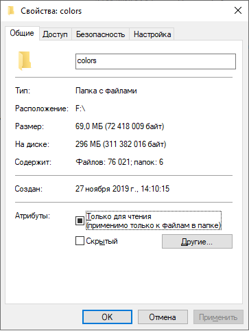
Fig 2.1 - Result of generating a training sample
Further, an m-file is created in the MATLAB application package, with the help of which the neural network will be trained.
clc;
%Выборка
path = 'D:\diploma\colors';
imds =imageDatastore(path,"IncludeSubfolders",true,"LabelSource","foldernames");
train = imds.splitEachLabel(1000,'randomize');
validation = imds.splitEachLabel(500,'randomize');
The script performs the following actions: clears the work area; the path by which the training sample can be found is indicated; parameters are indicated that indicate that the training sample is divided into subfolders and the names of the folders are the names of colors that will need to be determined in the future; 1000 examples are randomly selected from the training test for each color, directly for training the neural network itself; Also, for each color from the training splicing, 500 examples are randomly selected to check the results of training the neural network on data that this neural network has not seen before.
To design and use neural networks in an application package, you need the Deep Learning Toolbox package, which allows you to design a neural network in a graphical editor, after which you can create MATLAB code based on the created architecture, which is used to train neural networks.
Next, a neural network is created with the architecture shown in Fig. 2.2.
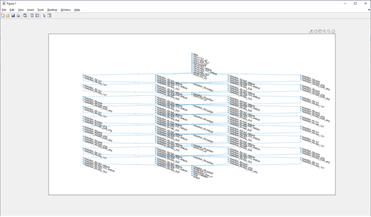
Fig 2.2 - Architecture of the created neural network
Next, the parameters of the neural network itself are set and training occurs, which was done using the following code:
net = trainNetwork(train,lgraph,options)
The neural network training process will be displayed on graphs, and every 50 iterations the results will be displayed on the command line. The results of training the neural network are presented in Fig. 2.3 and Fig. 2.4.
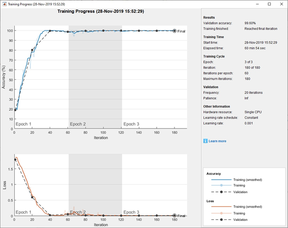
Fig 2.3 - Schedule of the NN learning process.
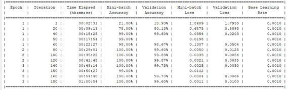
Fig 2.4 - Results of training neural network, displayed in the MATLAB command line
As a result, at the final iteration of NN training, the prediction accuracy on the validation data is 99.6%, which is sufficient to solve the problem.
Using the save (net, 'net') command, you can save the trained neural network and load it into the workspace when the program starts using the load (net) command.
To test the possibility of using the trained neural network for real problems, a photograph of the Rubik's cube was taken, shown in Fig. 2.5 and loaded into MATLAB.
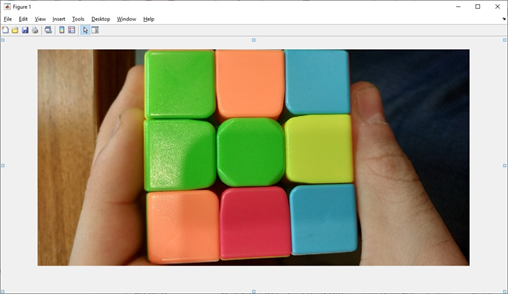
Fig 2.5 - Photo of the Rubik's cube.
Next, you need to accurately determine the colors of the elements of the Rubik's cube. For each element, an area of 140 by 140 pixels is selected, and the area data is alternately transmitted to the output of the NN. By feeding the region of the first element shown in Fig. 2.6, at the output it was obtained that with a probability of 1.0000 this is a green area.
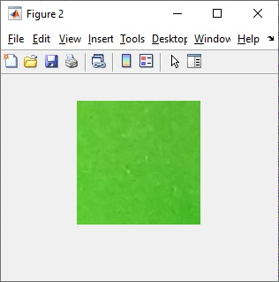
Fig 2.6 - The area of the first element of the Rubik's cube supplied to the input of the NN
Further, the regions shown in Fig. 2.7 and fig. 2.8. For these areas, the following results were obtained at the output: in Fig. 2.7 with a probability of 0.9998 - the area is orange, and in Fig. 2.8 with a probability of 0.9999 - blue area.
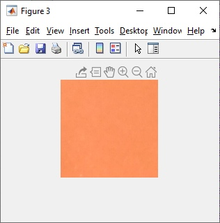
Fig 2.7 - The second area supplied to the input of the NN
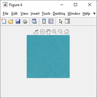
Fig 2.8 - The third area supplied to the input of the NN
The results of the work of the created neural network satisfy the set task and cope well with real data.
Conclusions
A vision system of a robotic arm with orthogonal grippers was designed.
The basic information about artificial neural networks is considered, the necessary minimum knowledge for the design of neural networks is stated.
Based on the data presented, an artificial convolutional neural network was designed, built and trained for recognizing the colors of Rubik's cube elements, which showed an excellent result of color determination and is now ready for use as part of a robotic arm with orthogonal grips, instead of the previously developed technical vision system, which is not has always shown good results.
List of sources
- Ф. Уоссерман. Нейрокомпьютерная техника: теория и практика/ под ред. А.И. Галушкина. М.: Мир. 1986.
- В.В.Круглов,В.В.Борисов.Искусственные нейронные сети.-М:Горячая линия.-Телеком,2001.-382с.
- Л.Г.Комарцова,А.В.Максимов.Нейрокомпьютеры.-Москва:МГТУ им.Баумана.2002.-320с.
- О.Г.Руденко, Е.В.Бодянский. Основы терии искусственных нейронних сетей.-Харьков:2002.-2002.-317с.
- В.Дьяконов,В.В.Круглов. Математические пакеты расширения МАТЛАБ.Специальный справочник.Спб:Питер.-2001.-480с.
- В.С.Медведев, В.Г.Потемкин. Нейронные сети.МАТЛАБ.-М:Диалог.-МИФИ.-2002.-496с.
- С.Осовский. Нейронные сети для обработки информации.Москва: Финансы и статистика .-2002.-344с.