Abstract
The term Deep Learning or Deep Neural Network refers to Artificial Neural Networks (ANN) with multi layers. Over the last few decades, it has been considered to be one of the most powerful tools, and has become very popular in the literature as it is able to handle a huge amount of data. The interest in having deeper hidden layers has recently begun to surpass classical methods performance in different fields; especially in pattern recognition. One of the most popular deep neural networks is the Convolutional Neural Network (CNN). It take this name from mathematical linear operation between matrixes called convolution. CNN have multiple layers; including convolutional layer, non-linearity layer, pooling layer and fullyconnected layer. The convolutional and fully- connected layers have parameters but pooling and non-linearity layers don't have parameters. The CNN has an excellent performance in machine learning problems. Specially the applications that deal with image data, such as largest image classification data set (ImageNet), computer vision, and in natural language processing (NLP) and the results achieved were very amazing . In this paper we will explain and define all the elements and important issues related to CNN, and how these elements work. In addition, we will also state the parameters that effect CNN efficiency. This paper assumes that the readers have adequate knowledge about both machine learning and artificial neural network.
Introduction
Convolutional Neural Network has had ground breaking results over the past decade in a variety of fields related to pattern recognition; from image processing to voice recognition. The most beneficial aspect of CNNs is reducing the number of parameters in ANN. This achievement has prompted both researchers and developers to approach larger models in order to solve complex tasks, which was not possible with classic ANNs. The most important assumption about problems that are solved by CNN should not have features which are spatially dependent. In other words, for example, in a face detection application, we do not need to pay attention to where the faces are located in the images. The only concern is to detect them regardless of their position in the given images. Another important aspect of CNN, is to obtain abstract features when input propagates toward the deeper layers. For example, in image classification, the edge might be detected in the first layers, and then the simpler shapes in the second layers, and then the higher level features such as faces in the next layers as shown in Fig. 1, as in [1, 3, 5, 15].
Convolutional Neural Network Elements
To obtain a good grasp of CNN, we start with its basic elements.
Convolution
Let’s assume that the input of our neural network has the presented shape in Fig. 2, It can be an image (e.g. color image of a CIFAR-10 dataset with a width and height of 32x32 pixels, and a depth of 3 which RGB channel) or a video (gray scale video whose height and width are the resolution, and the depth are the frames) or even an experimental video, which has width and height of (LxL) sensor values, and the depths are associated with different time frames, as in [2, 10, 15].
Why convolution? Let's assume that the network receives raw pixels as input. Therefore, to connect the input layer to only one neuron (e.g. in the hidden layer in the Multi-Layer perceptron), as an example, there should be 32x32x3 weight connections for the CIFAR-10 dataset.
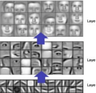
Fig. 1. Learned features from a Convolutional Neural Network
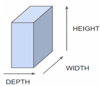
Fig. 2. Three dimensional Input representation of CNN
If we add one more neuron into the hidden layer, then we will need another 32x32x3 weight connection, which will become in total, 32x32x3x2 parameters. To make it clearer, more than 6000 weight parameters are used to connect the input to just only two nodes. It may be thought that two neurons might not be enough for any useful processing for an image classification application. To make it more efficient, we can connect the input image to the neurons in the next layer with exactly the same values for the height and width. It can be assumed this network is applied for the type of processing such as the edge in the image. However, the mentioned network needs 32x32x3 by 32x32 weight connections, which are (3,145,728), as in [4, 5, 14].
Therefore, looking for a more efficient method, it emerged that instead of a full connection, it is a good idea to look for local regions in the picture instead of in the whole image. Fig. 3, shows a regional connection for the next layer. In other words, the hidden neurons in the next layer only get inputs from the corresponding part of the previous layer. For example, it can only be connected to 5x5 neurons. Thus, if we want to have 32x32 neurons in the next layer, then we will have 5x5x3 by 32x32 connections which is 76,800 connections (compared to 3,145,728 for full connectivity), as in [1, 9, 13, 14, 17].
Although the size of connection drastically dropped, it still leaves so many parameters to solve. Another assumption for simplification, is to keep the local connection weights fixed for the entire neurons of the next layer. This will connect the neighbor neurons in the next layer with exactly the same weight to the local region of the previous layer. Therefore, it again drops many extra parameters, and reduces the number of weights to only 5x5x3=75 to connect 32x32x3 neurons to 32x32 in the next layer [5, 8, 11].
There are many benefits to these simple assumptions. Firstly, the number of connections decrease from around 3 million to only 75 connections in the presented example. Secondly, and a more interesting concept, is that fixing the weights for the local connections is similar to sliding a window of 5x5x3 in the input neurons and mapping the generated output to the corresponding place. It provides an opportunity to detect and recognize features regardless of their positions in the image. This is the reason why they are called convolutions [6, 7, 16].
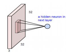
Fig. 3. Convolution as alternative for fully connected network
To show the astounding effect of the convolution matrix, Fig.4, depicts what will happen if we manually pick the connection weight in a 3x3 window.
As we can see Fig.4, the matrix can be set to detect edges in the image. These matrices are also called a filter because they act like the classic filters in the image processing. However, in the convolutional neural network these filters are initialized, followed by the training procedure shape filters, which are more suitable for the given task.
To make this method more beneficial, it is possible to add more layers after the input layer. Each layer can be associated with different filters. Therefore, we can extract different features from the given image. Fig. 5, shows how they are connected to the different layers. Each layer has its own filter and therefore extracts different features from the input. The neurons shown in Fig. 5, use a different filter, but look at the same part of the input image. [6, 8, 15, 17]
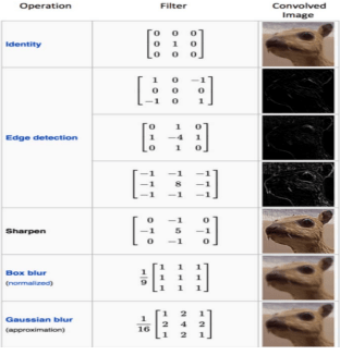
Fig.4. Effects of different convolution matrix
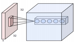
Fig. 5. Multiple layers which each of them correspond to different filter but looking at the same region in the given image
Stride
In fact, CNN has more options which provide a lot of opportunities to even decrease the parameters more and more, and at the same time reduce some of the side effects. One of these options is stride. In the above mentioned example, it is simply assumed that the next layer’s node has lots of overlaps with their neighbors by looking at the regions. We can manipulate the overlap by controlling the stride. Fig. 6, shows a given 7x7 image. If we move the filter one node every time, we can have a 5x5 output only. Note that the output of the three left matrices in Fig. 6, have an overlap (and three middle ones together and three right ones also). However, if we move and make every stride 2, then the output will be 3x3. Put simply, not only overlap, but also the size of the output will be reduced. [5, 12, 16].
Equation (1), formalize this, given the image NxN dimension and the filter size of the FxF, the output size O as shown in Fig. 7.

Where N is the input size, F is the filter size, and S is the stride size.
Padding
One of the drawbacks of the convolution step is the loss of information that might exist on the border of the image. Because they are only captured when the filter slides, they never have the chance to be seen. A very simple, yet efficient method to resolve the issue, is to use zero-padding. The other benefit of zero padding is to manage the output size. For example, in Fig. 6, with N=7 and F=3 and stride 1, the output will be 5x5 (which shrinks from a 7x7 input).

Fig. 6. Stride 1, the filter window moves only one time for each connection
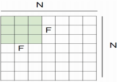
Fig. 7. The effect of stride in the output
However, by adding one zero-padding, the output will be 7?7, which is exactly the same as the original input (The actual N now becomes 9, use the formula (1). The modified formula including zero-padding is formula (2).

Where P is the number of the layers of the zero-padding (e.g. P=1 in Fig. 8), This padding idea helps us to prevent network output size from shrinking with depth. Therefore, it is possible to have any number of deep convolutional networks. [2, 12]
Feature of CNN
The weight sharing brings invariance translations to the model. It helps to filter the learn feature regardless of the spatial properties. By starting random values for the filters, they will learn to detect the edge (such as in Fig. 4) if it improves the performance. It is important to remember that if we need to know that something is spatially important in the given input, then it is an extremely bad idea to use a shared weight.
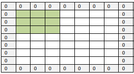
Fig. 8. Zero-padding

Fig. 9. Visualizing Convolutional deep neural network layers
This concept can be extended to different dimensions also. For example, if it is sequential data such as an audio, then it can employ a one dimensional audio. If it is an image, as it is shown, two dimensional convolutions can be applied. And for videos, or 3D images, a three dimensional convolution can be used. This simple idea beat all the classic object recognition methods in computer vision in the 2012 ImageNet challenge as shown in Fig. 9, [5, 14, 18]
Convolutional Formula
The convolution for one pixel in the next layer is calculated according to the formula (3).

Where net(i,j) is the output in the next layer, x is the input image and w is the kernel or filter matrix and * is the convolution operation. Fig. 10, shows how the convolution works. As can be seen, the element by element product of the input and kernel is aggregated, and then represents the corresponding point in the next layer. [4, 9]
Nonlinearity
The next layer after the convolution is non-linearity. The non-linearity can be used to adjust or cut-off the generated output. This layer is applied in order to saturate the output or limiting the generated output.
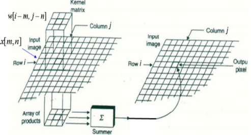
Fig. 10. Details on Convolution layer
For many years, sigmoid and tanh were the most popular non-linearity. Fig. 11, shows the common types of nonlinearity. However, recently, the Rectified Linear Unit (ReLU) has been used more often for the following reasons.
- ReLU has simpler definitions in both function and gradient.

- The saturated function such as sigmoid and tanh cause problems in the back propagation. As the neural network design is deeper, the gradient signal begins
to vanish, which is called the
vanishing gradient
. This happens since the gradient of those functions is very close to zero almost everywhere but the center. However, the ReLU has a constant gradient for the positive input. Although the function is not differentiable, it can be ignored in the actual implementation. - The ReLU creates a sparser representation. because the zero in the gradient leads to obtaining a complete zero. However, sigmoid and tanh always have non-zero results from the gradient, which might not be in favor for training. [2, 5, 13]
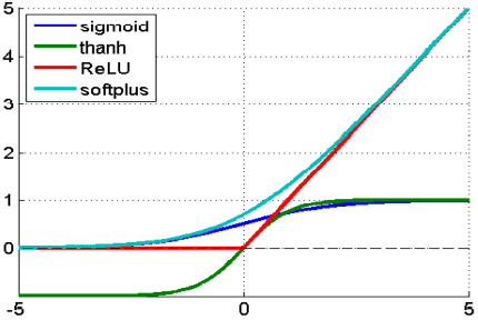
Fig. 11. Common types of nonlinearity
Pooling
The main idea of pooling is down-sampling in order to reduce the complexity for further layers. In the image processing domain, it can be considered as similar to reducing the resolution. Pooling does not affect the number of filters. Max-pooling is one of the most common types of pooling methods. It partitions the image to sub-region rectangles, and it only returns the maximum value of the inside of that sub-region. One of the most common sizes used in max-pooling is 2x2. As can see in Fig. 12, when pooling is performed in the top-left 2x2 blocks (pink area), it moves 2 and focus on top-right part. This means that stride 2 is used in pooling. To avoid down-sampling, stride 1 can be used, which is not common. It should be considered that down-sampling does not preserve the position of the information. Therefore, it should be applied only when the presence of information is important (rather than spatial information). Moreover, pooling can be used with non-equal filters and strides to improve the efficiency. For example, a 3x3 max-pooling with stride 2 keeps some overlaps between the areas. [5, 10, 16]
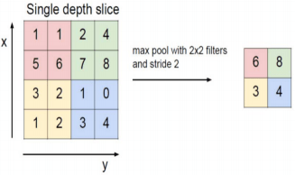
Fig. 12. Max-pooling is demonstrated. The max-pooling with 2x2 filter and stride 2 lead to down-sampling of each 2x2 blocks is mapped to 1 block (pixel).
Fully-Connected Layer
The fully-connected layer is a similar to the way that neurons are arranged in a traditional neural network. Therefore, each node in a fully-connected layer is directly connected to every node in both the previous and in the next layer as shown in Fig. 13, From this figure we can note that each of the nodes in the last frames in the pooling layer are connected as a vector to the first layer from the fully-connected layer. These are the most parameters used with the CNN within these layers, and take a long time in training [3, 8].
The major drawback of a fully-connected layer, is that it includes a lot of parameters that need complex computational in training examples. Therefore, we try to eliminate the number of nodes and connections. The removed nodes and connection can be satisfied by using the dropout technique. For example, LeNet and AlexNet designed a deep and wide network while keeping the computational complex constant [4, 6, 9].
The essence of the CNN network, which is the convolution, is when the nonlinearity and pooling layer are introduced. Most common architecture uses three of them as
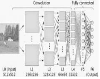
Fig. 13. Fully-Connected Layer
Popular CNN Architecture
LeNet
LeNet was introduced by Yan LeCun for digit recognition Fig. 14., It includes 5 convolutional layers and one fully connected layer (like MLP). [8, 19]

Fig. 14. LeNet introduced by Yan LeCun
AlexNet
AlexNet contains 5 convolutional layers as well as 2 fully connected layers for learning features Fig. 15, It has max-pooling after the first, second and fifth convolutional layer. In total it has 650K neurons, 60M parameters, and 630M connections. The AlexNet was the first to show deep learning was effective in computer vision tasks. [2, 7]

Fig. 15. AlexNet introduced by Krizhevsky 2014
Conclusion
In this paper we discuss the important issues that related Convolutional Neural Network (CNN) and explain the effect each parameter on performance of network . The most important layer in CNN is convolution layer Which takes most of the time within the network. Network performance also depends on the number of levels within the network. But in the other hand as the number of levels increases the time required to train and test the network. Today the CNN consider as power full tool within machine learning for a lot of application such as face detection and image , video recognitions and voice recognition.
References
- O. Abdel-hamid, L. Deng, and D. Yu, “Exploring Convolutional Neural Network Structures and Optimization Techniques for Speech Recognition, ” no. August, pp. 3366–3370, 2013.
- http://www.deeplearningbook.org/contents...
- V. Dumoulin and F. Visin, “A guide to convolution arithmetic for deep learning,” pp. 1–28, 2016.
- Y. Guo, Y. Liu, A. Oerlemans, S. Wu, and M. S. Lew, “Author ’ s Accepted Manuscript Deep learning for visual understanding : A review To appear in : Neurocomputing,” 2015.
- https://www.opendatascience.com/blog/....
- I. Kokkinos, E. C. Paris, and G. Group, “Introduction to Deep Learning Convolutional Networks, Dropout, Maxout 1,” pp. 1–70.
- Krizhevsky, A., Sutskever, I. and Hinton, G.E., 2012. Imagenet classification with deep convolutional neural networks. In Advances in neural information processing systems (pp. 1097- 1105).
- N. Kwak, “Introduction to Convolutional Neural Networks ( CNNs ),” 2016.
- O. Russakovsky, J. Deng, H. Su, J. Krause, S. Satheesh, S. Ma, Z. Huang, A. Karpathy, C. V Jan, J. Krause, and S. Ma, “ImageNet Large Scale Visual Recognition Challenge.”.
- D. Stutz and L. Beyer, “Understanding Convolutional Neural Networks,” 2014.
- C. Szegedy, W. Liu, Y. Jia, P. Sermanet, S. Reed, D. Anguelov, D. Erhan, V. Vanhoucke, and A. Rabinovich, “Going Deeper with Convolutions,” 2014.
- K. Teilo, “ An Introduction to Convolutional Neural Networks,” no. NOVEMBER 2015, pp. 0–11, 2016.
- R. E. Turner, “Lecture 14 : Convolutional neural networks for computer vision,” 2014.
- J. Wu, “Introduction to Convolutional Neural Networks,” pp. 1–28, 2016.
- https://ujjwalkarn.me/2016/08/11/...
- http://www.slideshare.net/hanneshapke/....
- Wei Xiong , Bo Du, Lefei Zhang, Ruimin Hu, Dacheng Tao "Regularizing Deep Convolutional Neural Networks with a Structured Decorrelation Constraint ” IEEE 16th International Conference on Data Mining (ICDM) , pp. 3366–3370, 2016.
- Taigman, Y., Yang, M., Ranzato, M.A. and Wolf, L., 2014. Deepface: Closing the gap to human-level performance in face verification. In Proceedings of the IEEE Conference on Computer Vision and Pattern Recognition (pp. 1701-1708).
- LeCun, Y., Bottou, L., Bengio, Y. and Haffner, P., 1998. Gradientbased learning applied to document recognition. Proceedings of the
IEEE, 86(11), pp.2278-2324.