 .
.
Laboratoire d'Electrotechnique et d'Electronique Industrielle; Laboratoire d'Electronique de l'Ecole Superieure de Physique et de Chimie Industrielles, France, 1999
Undersampling for the training of feedback neural networks on large sequences; application to the modeling of an induction machine
(Shortened version of the article)
Full version of the article (original): http://www.esa.espci.fr/ARTICLES/1999pafo.pdf
L. Constant, B. Dagues, I. Rivals, L. Personnaz
Abstract
This paper proposes an economic method for the nonlinear modeling of dynamic processes using feedback neural networks, by undersampling the training sequences. The undersampling (i) allows a better exploration of the operating range of the process for a given size of the training sequences, and (ii) it speeds up the training of the feedback networks. This
method is successfully applied to the training of a neural model of the electromagnetic part of an induction machine, whose sampling period must be small enough to take fast variations of the input voltage into account, i.e. smaller than 1  .
.
1. Introduction
We are interested in the real-time emulation of systems consisting of a static converter, an induction machine, and of the associated sensors [1]. Implementations of classic induction machine models are computationally intensive, which prevents real-time processing. The ability to parsimoniously approximate nonlinear mappings, as well as the possibility of parallel computing, make neural networks efficient in terms of accuracy and computation time, and make their use interesting in this context. This paper thus presents the neural modeling [2] [3] of the electromagnetic part of an induction machine [4] [5] [6]. A difficulty of this type of dynamic modeling is the design of training sequences exploring the entire range of operation of the induction machine. Moreover, even if the dynamics of the induction machine itself does not necessitate a very high sampling frequency, the latter should be high enough to take fast variations of the input voltage into account, constraint which leads to huge training sequences. Under these conditions, the training is not easily achievable from the point of view both of its duration and of its success, due to local minima. To overcome these problems, we propose (i) to undersample the training sequences, and (ii) to perform an adequate modification of the parameters obtained after training so that the feedback neural model finally operates at the desired, higher, sampling frequency. Thanks to this method, it is possible for a given number of samples to explore a larger portion of the range of operation of the process, i.e. to make the training sequences more informative, and to perform a more efficient training.
2. Neural modeling of an induction machine
This section introduces the process (simulated induction machine) to be modeled, the neural model architecture, and the training procedure used to estimate the network parameters.
2.1. Reference model
The simulated process is based on the classic two-phase model of an induction machine with a three-phase stator, P pairs of poles and a squirrel-cage rotor. The two-phase model in the reference frame ( ,
,  ) fixed on the stator consists of:
- a system Of differential equations for the fluxes:
 , (1)
, (1)
- a relation between the fluxes and the electro-magnetic torque:
 , (2)
, (2)
- relations between the fluxes and the stator currents:
 , (3)
, (3)
A discrete-time model is obtained by discretizing the above continuous-time model using the Runge-Kutta method of order 4. This discrete-time model, termed "reference model", is used to generate training and test sequences for the neural model.
2.2. Neural model architecture
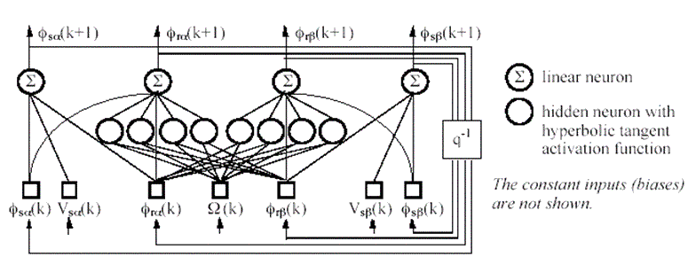
The neural network architecture is based on the equations of the two-phase model, and consists thus of two distinct parts. The first one, a feedback (dynamic) input-output neural network shown in Fig. 1, corresponds to the system of differential equations for the fluxes (1).

Fig. 1: Feedback neural model of the induction machine electromagnetic part.
Its state outputs are the 4 fluxes, which are computed according to the stator voltages, the mechanical speed, and the fluxes at the previous time step. According to the reference model, the 2 stator fluxes are estimated by two linear functions, and the 2 rotor fluxes are estimated by 2 nonlinear subnetworks.
These subnetworks have only the input variables involved in the corresponding differential equations, a layer of 4 hidden neurons with hyperbolic tangent activation function, and a linear output neuron. The second part of the neural model is a feedforward (static) neural network, which implements relations (2) and (3): it computes the stator currents and the electromagnetic torque according to the fluxes [4]. The training of the feedforward network being independent from the sampling period, we focus here on the training of the feedback network.
2.3. Training on undersampled sequences
A very small sampling period is not necessary to obtain an accurate discretization of the continuous-time model of the electromagnetic part of the induction machine, but at the end, the induction machine model must be associated to a static converter model. Phenomena such as the dead-times of the converter must thus be taken into account, so that the working sampling period must be at most of 1  . The design of an appropriate training sequence mainly necessitates the determination of the domain defined by the ranges of mechanical speed, flux amplitude, and load torque that must be explored in the training sequence so that the network is able to reproduce unlearned modes of operation. In [7], such a training sequence has been designed. The latter being extremely large (it consists of hundreds of thousands of samples), it is undersampled here at 10
  for the training of the neural model. The training is performed in an undirected (parallel) fashion using an iterative non recursive quasi - Newtonian algorithm; the gradient of the cost-function is computed by backpropagation [2] [3]. Section 3 presents how the network parameters values obtained after training can be modified so that the network operates at the desired sampling period, i.e. 1
  .
.
3. Sampling period modification
We suppose that a SISO first-order nonlinear discrete-time predictive model of an unknown continuous-time process has been obtained using measurements at a sampling period T:
 , (4)
, (4)
where f is a nonlinear function. The problem is to derive from (4) a discrete-time model working at a smaller sampling period T':
 , (5)
, (5)
For this purpose, we propose to consider that the discrete-time model (4) is a discretization of the following fictitious continuous-time model (6) with one of the usual discretization rules:
 , (6)
, (6)
Subsection 3.1 determines which discretization rules allow the computation of a', b', c' from a, b, c.
3.1. Possible discretization rules
We search for the discretization rules on which it is possible to base a transformation of the discrete-time model (4) into the discrete-time model (5).
a) Euler’s backward rule
The approximate discretization of (6) using Euler’s backward rule is obtained by assuming that dy/dt is constant between kT and (k+1)T, and that it is equal to F (kT). Hence the model for a sampling period T:
 , (7)
, (7)
Performing Euler at T', and eliminating ac, bc, cc with (7), one obtains:
 , (8)
, (8)
b) Euler’s forward rule
The discretization using Euler’s forward rule is obtained by assuming that dy/dt is constant between kT and (k+1)T, and equal to F((k+1)T). Because of the non-linearity f in F, an explicit difference equation is generally impossible to derive (for instance if f is implemented by nonlinear neurons). This rule is thus not suited to our problem.
c) Tustin’s (trapezoidal) rule
For the same reason as for Euler’s forward rule, this rule is also not suited to our problem.
d) Other rules
For a linear model, there exist many other rules to derive a discrete-time transfer function [8], in particular those leading to a behavior of the discrete-time system that is identical to that of the continuous-time system at the sampling instants for a given type of input (impulse, step, ramp, sinusoid, etc.). Unfortunately, there is no general rule for exact matching even for specific inputs in the nonlinear case. To conclude, the only rule that can generically be used for our problem is Euler’s backward rule.
3.2. Application to feedback neural networks
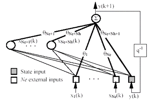
For simplicity, we consider a first-order feedback network with Ne external inputs (possibly including a constant unit input), a layer of Nh nonlinear neurons, and a linear state output with direct connections to the inputs (see Fig. 2).

Fig. 2: Feedback neural network of order 1.
We denote the external inputs at time k by  for i=1 to Ne, and the outputs of the hidden neurons by
  for i=1 to Nh. The elements of the parameter vector
  corresponding to all the connections to the output are numbered as in Fig 2. The network behavior is described by:
 , (9)
, (9)
We look for the parameters  ' of the output neuron of the network working at a smaller sampling period T'. This network behavior is by definition described by:
 , (10)
As shown in the previous section, Euler’s backward rule can be used to derive the parameters  ':
':
 , (11)
 , (12)
The elements of  and
and  ' corresponding to the connections from the inputs to the hidden neurons are identical. This transformation is easily generalized to the case of a state-space neural network [3] with several states: for each state output neuron, the parameter of the connection from the corresponding state input is modified according to (11), and all the others according to (12).
References