Source:http://research.microsoft.com/copyright/accept.asp?path=http://research.microsoft.com/~hoppe/recon.pdf&pub=acm
Surface Reconstruction from Unorganized Points
Hugues Hoppe Tony DeRose Tom Duchamp John McDonald Werner Stuetzle
University of Washington Seattle, WA 98195
Abstract
We describe and demonstrate an algorithm that takes as input an unorganized set of points  or near an unknown manifold M, and produces as output a simplicial surface that approximates M. Neither the topology, the presence of boundaries, nor the geometry of M are assumed to be known in advance — all are inferred automatically from the data. This problem naturally arises in a variety of practical situations such as range scanning an object from multiple view points, recovery of biological shapes from two-dimensional slices, and interactive surface sketching.
CR Categories and Subject Descriptors: I.3.5 [Computer Graphics]: Computational Geometry and Object Modeling.
Additional Keywords: Geometric Modeling, Surface Fitting, Three-Dimensional Shape Recovery, Range Data Analysis.
1 Introduction
Broadly speaking, the class of problems we are interested in can be stated as follows: Given partial information of an unknown surface, construct, to the extent possible, a compact representation of the surface. Reconstruction problems of this sort occur in diverse scienti c and engineering application domains, including:
Surfaces from range data: The data produced by laser range scanning systems is typically a rectangular grid of distances from the sensor to the object being scanned. If the sensor and object are fixed, only objects that are “point viewable” can be fully digitized. More sophisticated systems, such as those produced by Cyberware Laboratory, Inc., are capable of digitizing cylindrical objects by rotating either the sensor or the object. However, the scanning of topologically more complex objects, including those as simple as a coffee cup with a handle (a surface of genus 1), or the object depicted in Figure 1a (a surface of genus 3), cannot be accomplished by either of these methods. To adequately scan these objects, multiple view points must be used. Merging the data generated from multiple view points to reconstruct a polyhedral surface representation is a non-trivial task [11].
Surfaces from contours: In many medical studies it is common to slice biological specimens into thin layers with a mi-crotome. The outlines of the structures of interest are then digitized to create a stack of contours. The problem is to reconstruct the three-dimensional structures from the stacks of two-dimensional contours. Although this problem has received a good deal of attention, there remain severe limitations with current methods. Perhaps foremost among these is the dif culty of automatically dealing with branching structures [3, 12].
Interactive surface sketching: A number of researchers, including Schneider [21] and Eisenman [6], have investigated the creation of curves in IR2 by tracing the path of a stylus or mouse as the user sketches the desired shape. Sachs et al. [19] describe a system, called 3-Draw, that permits the creation of free-form curves in IR3 by recording the motion of a stylus tted with a Polhemus sensor. This can be extended to the design of free-form surfaces by ignoring the order in which positions are recorded, allowing the user to move the stylus arbitrarily back and forth over the surface. The problem is then to construct a surface representation faithful to the unordered collection of points.
Reconstruction algorithms addressing these problems have typically been crafted on a case by case basis to exploit partial structure in the data. For instance, algorithms solving the surface from contours problem make heavy use of the fact that data are organized into contours (i.e., closed polygons), and that the contours lie in parallel planes. Similarly, specialized algorithms to reconstruct surfaces from multiple view point range data might exploit the adjacency relationship of the data points within each view.
In contrast, our approach is to pose a unifying general problem that does not assume any structure on the data points. This approach has both theoretical and practical merit. On the theoretical side, abstracting to a general problem often sheds light on the truly critical aspects of the problem. On the practical side, a single algorithm that solves the general problem can be used to solve any speci c problem instance.
1.1 Terminology
By a surface we mean a “compact, connected, orientable two-dimensional manifold, possibly with boundary, embedded in IR3” (cf. O’Neill [17]). A surface without boundary will be called a closed surface. If we want to emphasize that a surface possesses a non-empty boundary, we will call it a bordered surface. A piecewise linear surface with triangular faces will be referred to as a simplicial surface. We use to denote the Euclidean length of a vector , and we use d(X Y) to denote the Hausdorff distance between the sets of points X and Y (the Hausdorff distance is simply the distance between the two closest points of X and Y).
Let X = 1 n be sampled data points on or near an unknown surface M (see Figure 1b). To capture the error in most sampling processes, we assume that each of the points i X is of the form i =i +i, wherei M is a point on the unknown surface and i IR3is an error vector. We call such a sample X -noisy if i for all i. A value for can be estimated in most applications (e.g., the accuracy of the laser scanner). Features of M that are small compared to will obviously not be recoverable.
It is also impossible to recover features of M in regions where insuf cient sampling has occurred. In particular, if M is a bordered surface, such as a sphere with a disc removed, it is impossible to distinguish holes in the sample from holes in the surface. To capture the intuitive notion of sampling density we need to make another de nition: Let Y = 1 n M be a (noiseless) sample of a surface M. The sample Y is said to be -dense if any sphere with radius and center in M contains at least one sample point in Y. A -noisy sample 1 n IR3of a surface M is said to be -dense if there exists a noiseless -dense sample 1 n M such that i =i +i,i , i = 1 n.
1.2 Problem Statement
The goal of surface reconstruction is to determine a surface M (see Figure 2f) that approximates an unknown surface M (Figure 1a), using a sample X (Figure 1b) and information about the sampling process, for example, bounds on the noise magnitude and the sampling density .
We are currently working to develop conditions on the original surface M and the sample X that are suf cient to allow M to be reliably reconstructed. As that work is still preliminary, we are unable to give guarantees for the algorithm presented here. However, the algorithm has worked well in practice where the results can be compared to the original surface (see Section 4).
2 Related Work
2.1 Surface Reconstruction
Surface reconstruction methods can be classi ed according to the way in which they represent the reconstructed surface.
Implicit reconstruction methods attempt to nd a smooth function f : IR3IR such that 1 n is close to the zero set Z(f ). They differ with respect to the form of f and the measure of closeness. Pratt [18] and Taubin [25] minimize the sum of squared Hausdorff distances from the data points to the zero set of a polynomial in three variables. Muraki [15] takes f to be a linear combination of three-dimensional Gaussian kernels with different means and spreads. His goodness-of- t function measures how close the values of f at the data points are to zero, and how well the unit normals to the zero set of f match the normals estimated from the data. Moore and Warren [13] t a piecewise polynomial recursively and then enforce continuity using a technique they call free form blending.
In contrast to implicit reconstruction techniques, parametric reconstruction techniques represent the reconstructed surface as a topological embedding f ( ) of a 2-dimensional parameter domain into IR3. Previous work has concentrated on domain spaces with simple topology, i.e. the plane and the sphere. Hastie and Stuet-zle [9] and Vemuri [26, 27] discuss reconstruction of surfaces by a topological embedding f ( ) of a planar region into IR3. Schudy and Ballard [22, 23] and Brinkley [4] consider the reconstruction of surfaces that are slightly deformed spheres, and thus choose to be a sphere. Sclaroff and Pentland [24] describe a hybrid implicit/parametric method for tting a deformed sphere to a set of points using deformations of a superquadric.
Compared to the techniques mentioned above, our method has several advantages:
It requires only an unorganized collection of points on or near the surface. No additional information is needed (such as normal information used by Muraki’s method).
Unlike the parametric methods mentioned above, it can reconstruct surfaces of arbitrary topology.
Unlike previously suggested implicit methods, it deals with boundaries in a natural way, and it does not generate spurious surface components not supported by the data.
2.2 Surface Reconstruction vs Function Reconstruction
Terms like “surface tting” appear in reference to two distinct classes of problems: surface reconstruction and function reconstruction. The goal of surface reconstruction was stated earlier. The goal of function reconstruction may be stated as follows: Given a surface M, a set i M , and a set yi IR , determine a function f : M IR, such that f ( i)yi.
The domain surface M is most commonly a plane embedded in IR3, in which case the problem is a standard one considered in approximation theory. The case where M is a sphere has also been extensively treated (cf. [7]). Some recent work under the title surfaces on surfaces addresses the case when M is a general curved surface such as the skin of an airplane [16].
Function reconstruction methods can be used for surface reconstruction in simple, special cases, where the surface to be reconstructed is, roughly speaking, the graph of a function over a known surface M. It is important to recognize just how limited these special cases are — for example, not every surface homeomorphic to a sphere is the graph of a function over the sphere. The point we want to make is that function reconstruction must not be misconstrued to solve the general surface reconstruction problem.
3 A Description of the Algorithm
3.1 Overview
Our surface reconstruction algorithm consists of two stages. In the rst stage we de ne a function f : D IR, where D IR3is a region near the data, such that f estimates the signed geometric distance to the unknown surface M. The zero set Z(f ) is our estimate for M. In the second stage we use a contouring algorithm to approximate Z(f ) by a simplicial surface.
Although the unsigned distance function f would be easier to estimate, zero is not a regular value of f . Zero is, however, a regular value of f , and the implicit function theorem thus guarantees that our approximation Z(f ) is a manifold.
The key ingredient to de ning the signed distance function is to associate an oriented plane with each of the data points. These
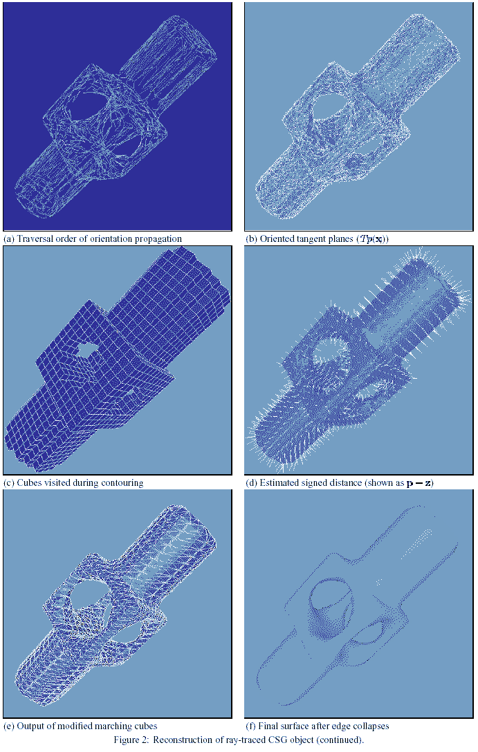
tangent planes serve as local linear approximations to the surface. Although the construction of the tangent planes is relatively simple, the selection of their orientations so as to de ne a globally consistent orientation for the surface is one of the major obstacles facing the algorithm. As indicated in Figure 2b, the tangent planes do not directly de ne the surface, since their union may have a complicated non-manifold structure. Rather, we use the tangent planes to de ne the signed distance function to the surface. An example of the simplicial surface obtained by contouring the zero set of the signed distance function is shown in Figure 2e. The next several sections develop in more detail the successive steps of the algorithm.
3.2 Tangent Plane Estimation
The first step toward defining a signed distance function is to compute an oriented tangent plane for each data point. The tangent plane
( i) associated with the data pointi is represented as a pointi,
called the center, together with a unit normal vector i. The signeddistance of an arbitrary point IR3to ( i) is de ned to be disti() = ( i)i. The center and normal for( i) are determined by gathering together the k points of X nearest to i; this set
is denoted by ( i) and is called thek-neighborhood ofi. (We
currently assume k to be a user-speci ed parameter, although in Section 5 we propose a method for determining k automatically.) The center and unit normal are computed so that the plane disti() = 0 is the least squares best tting plane to ( i). That is, the center i is taken to be the centroid of ( i), and the normali
is determined using principal component analysis. To compute i,
the covariance matrix of ( i) is formed. This is the symmetric
3 3 positive semi-definite matrix

where X denotes the outer product vector operator1. If 3 denote the eigenvalues of CV associated with unit eigenvectors, respectively, we choosei to be eitheri i . The
selection determines the orientation of the tangent plane, and it must be done so that nearby planes are “consistently oriented”.
3.3 Consistent Tangent Plane Orientation
Suppose two data points i j X are geometrically close. Ideally, when the data is dense and the surface is smooth, the corresponding
tangent planes ( i) = (i i) and( j) = (j j) are nearly
parallel, i.e. i j 1. If the planes are consistently oriented, then i j +1; otherwise, either i orj should be ipped.The dif culty in nding a consistent global orientation is that this condition should hold between all pairs of “suf ciently close” data points.
We can model the problem as graph optimization. The graph
contains one node Ni per tangent plane( i), with an edge (i j)between Ni andNj if the tangent plane centersi andj are sufficiently close (we will be more precise about what we mean by suf ciently close shortly). The cost on edge (i j) encodes the degree to which Ni andNj are consistently oriented and is taken to bei j. The problem is then to select orientations for the tangent planes so as to maximize the total cost of the graph. Unfortunately, this problem can be shown to be NP-hard via a reduction to MAX-CUT [8]. To ef ciently solve the orientation problem we must therefore resort to an approximation algorithm.
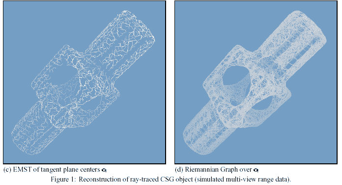
Before describing the approximation algorithm we use, we must decide when a pair of nodes are to be connected in the graph. Since the surface is assumed to consist of a single connected component, the graph should be connected. A simple connected graph for a set of points that tends to connect neighbors is the Euclidean Minimum Spanning Tree (EMST). However, the EMST over the tangent plane centers 1 n (Figure 1c) is not suf ciently dense in edges to serve our purposes. We therefore enrich it by adding a number of edges to it. Speci cally, we add the edge (i j) if either i is
in the k-neighborhood of j, orj is in the k-neighborhood ofi
(where k-neighborhood is defined over 1 n as it was for X). The resulting graph (Figure 1d), called the Riemannian Graph, is thus constructed to be a connected graph that encodes geometric proximity of the tangent plane centers.
A relatively simple-minded algorithm to orient the planes would be to arbitrarily choose an orientation for some plane, then “propagate” the orientation to neighboring planes in the Riemannian Graph. In practice, we found that the order in which the orientation is propagated is important. Figure 3b shows what may result when propagating orientation solely on the basis of geometric proximity; a correct reconstruction is shown in Figure 3c. Intuitively, we would like to choose an order of propagation that favors propagation from
( i) to( j) if the unoriented planes are nearly parallel. This
can be accomplished by assigning to each edge (i j) in the Rieman-
nian Graph the cost 1 i j . In addition to being non-negative,
this assignment has the property that a cost is small if the unoriented tangent planes are nearly parallel. A favorable propagation order can therefore be achieved by traversing the minimal spanning tree (MST) of the resulting graph. This order is advantageous because it tends to propagate orientation along directions of low curvature in the data, thereby largely avoiding ambiguous situations encountered when trying to propagate orientation across sharp edges (as at the tip of the cat’s ears in Figure 3b). In the MST shown in Figure 2a, the edges are colored according to their cost, with the brightly colored edges corresponding to regions of high variation (where i j issomewhat less than 1).
To assign orientation to an initial plane, the unit normal of the plane whose center has the largest z coordinate is forced to point toward the +z axis. Then, rooting the tree at this initial node, we traverse the tree in depth- rst order, assigning each plane an orientation that is consistent with that of its parent. That is, if during traversal, the current plane ( i) has been assigned the
orientation i and( j) is the next plane to be visited, thenj is
replaced with j ifi j 0.
This orientation algorithm has been used in all our examples and has produced correct orientations in all the cases we have run. The resulting oriented tangent planes are represented as shaded rectangles in Figure 2b.
3.4 Signed Distance Function
The signed distance f ( ) from an arbitrary point IR3to a known surface M is the distance between and the closest point M, multiplied by 1, depending on which side of the surface lies. In reality M is not known, but we can mimic this procedure using the oriented tangent planes as follows. First, we nd the tangent plane ( i) whose centeri is closest to. This tangent plane is a local linear approximation to M, so we take the signed distance f ( ) to M to be the signed distance between and its projection
onto ( i); that is,

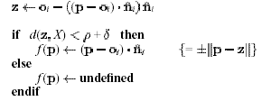
If M is known not to have boundaries, this simple rule works well. However, the rule must be extended to accommodate surfaces that might have boundaries. Recall that the set X = 1 n is assumed to be a -dense, -noisy sample of M. If there was no noise, we could deduce that a point with d( X) cannot be
a point of M since that would violate X being -dense. Intuitively, the sample points do not leave holes of radius larger than . If the sample is -noisy, the radius of the holes may increase, but by no more than . We therefore conclude that a point cannot be a point of M if d( X) + . If the projection of onto the closest tangent plane has d( X) + , we take f ( ) to be unde ned. Unde ned values are used by the contouring algorithm of Section 3.5 to identify boundaries.
Stated procedurally, our signed distance function is de ned as:
i index of tangent plane whose center is closest to
{Compute z as the projection of p onto Tp(xi)}

The simple approach outlined above creates a zero set Z(f ) that is piecewise linear but contains discontinuities. The discontinuities result from the implicit partitioning of space into regions within which a single tangent plane is used to de ne the signed distance function. (These regions are in fact the Voronoi regions associated
with the centers i.) Fortunately, the discontinuities do not adversely
affect our algorithm. The contouring algorithm discussed in the next section will discretely sample the function f over a portion of a 3-dimensional grid near the data and reconstruct a continuous piecewise linear approximation to Z(f ).
3.5 Contour Tracing
Contour tracing, the extraction of an isosurface from a scalar function, is a well-studied problem [1, 5, 28]. We chose to implement a variation of the marching cubes algorithm (cf. [1]) that samples the function at the vertices of a cubical lattice and nds the contour intersections within tetrahedral decompositions of the cubical cells.
To accurately estimate boundaries, the cube size should be set so that edges are of length less than + . In practice we have often found it convenient to set the cube size somewhat larger than this value, simply to increase the speed of execution and to reduce the number of triangular facets generated.
The algorithm only visits cubes that intersect the zero set by pushing onto a queue only the appropriate neighboring cubes (Figure 2c). In this way, the signed distance function f is evaluated only at points close to the data. Figure 2d illustrates the signed distance function by showing line segments between the query points (at the cube vertices) and their associated projected points . As suggested in Section 3.4, no intersection is reported within a cube if the signed distance function is unde ned at any vertex of the cube, thereby giving rise to boundaries in the simplicial surface.
The resulting simplicial surface can contain triangles with arbitrarily poor aspect ratio (Figure 2e). We alleviate this problem using a post-processing procedure that collapses edges in the surface using an aspect ratio criterion.2The nal result is shown in Figure 2f. Alternatively, other contouring methods exist that can guarantee bounds on the triangle aspect ratio [14].
4 Results
We have experimented with the reconstruction method on data sets obtained from several different sources. In all cases, any structure (including ordering) that might have been present in the point sets was discarded.
Meshes : Points were randomly sampled from a number of existing simplicial surfaces3. For instance, the mesh of Figure 3a was randomly sampled to yield 1000 unorganized points, and these in turn were used to reconstruct the surface in Figure 3c. This particular case illustrates the behavior of the method on a bordered surface (the cat has no base and is thus homeomorphic to a disc). The reconstructed knot (original mesh from Rob Scharein) of Figure 3d is an example of a surface with simple topology yet complex geometrical embedding.
Ray Traced Points : To simulate laser range imaging from multiple view points, CSG models were ray traced from multiple eye points. The ray tracer recorded the point of rst intersection along each ray. Eight eye points (the vertices of a large cube centered at the object) were used to generate the point set of Figure 1b from the CSG object shown in Figure 1a. This is the point set used in Section 3 to illustrate the steps of the algorithm (Figures 1a-2f).
Range Images : The bust of Spock (Figure 3e) was reconstructed from points taken from an actual cylindrical range image (generated by Cyberware Laboratory, Inc.). Only 25 of the original points were used.
Contours : Points from 39 planar (horizontal) slices of the CT scan of a femur were combined together to obtain the surface of Figure 3f.
The algorithm’s parameters are shown in the next table for each of the examples. The execution times were obtained on a 20 MIPS workstation. The parameter + and the marching cube cell size are both expressed as a fraction of the object’s size. The parameter + is set to in nity for those surfaces that are known to be closed.
Object |
n |
k |
ro+delta |
cell size |
time |
|
|
|
|
|
(seconds) |
cat |
1000 |
15 |
.06 |
1 30 |
19 |
knot |
10000 |
20 |
|
1 50 |
137 |
mechpart |
4102 |
12 |
|
1 40 |
54 |
spock |
21760 |
8 |
.08 |
1 80 |
514 |
femur |
18224 |
40 |
.06 |
1 50 |
2135 |
5 Discussion
5.1 Tangent Plane Approximation
The neighborhood ( i) of a data pointi is de ned to consist
of its k nearest neighbors, where k is currently assumed to be an input parameter. In the case where the data contains little or no noise, k is not a critical parameter since the output has been empirically observed to be stable over a wide range of settings. However, it would be best if k could be selected automatically. Furthermore, allowing k to adapt locally would make less stringent the requirement that the data be uniformly distributed over the surface. To select and adapt k, the algorithm could incrementally gather points while monitoring the changing eigenvalues of the covariance matrix (see Section 3.2). For small values of k, data noise tends to dominate, the eigenvalues are similar, and the eigenvectors do not reveal the surface’s true tangent plane. At the other extreme, as k becomes
large, the k-neighborhoods become less localized and the surface curvature tends to increase the “thickness” 3
i of the neighborhood.
Another possible criterion is to compare 3
i to some local or global
estimate of data noise. Although we have done some initial experimentation in this direction, we have not yet fully examined these options.
If the data is obtained from range images, there exists some knowledge of surface orientation at each data point. Indeed, each data point is known to be visible from a particular viewing direction, so that, unless the surface incident angle is large, the point’s tangent plane orientation can be inferred from that viewing direction. Our method could exploit this additional information in the tangent plane orientation step (Section 3.3) by augmenting the Riemannian Graph with an additional pseudo-node and n additional edges.
5.2 Algorithm Complexity
A spatial partitioning Abstract Data Type greatly improves performance of many of the subproblems discussed previously. The critical subproblems are (with their standard time complexity):
EMST graph (O(n2)) k-nearest neighbors to a given point (O(n + k log n)) nearest tangent plane origin to a given point (O(n))
Hierarchical spatial partitioning schemes such as octrees [20] and k-D trees [2] can be used to solve these problems more ef- ciently. However, the uniform sampling density assumed in our data allows simple spatial cubic partitioning to work ef ciently. The axis-aligned bounding box of the points is partitioned by a cubical grid. Points are entered into sets corresponding to the cube to which they belong, and these sets are accessed through a hash table indexed by the cube indices. It is dif cult to analyze the resulting improvements analytically, but, empirically, the time complexity of the above problems is effectively reduced by a factor of n, except for the k-nearest neighbors problem which becomes O(k).
As a result of the spatial partitioning, the Riemannian Graph can be constructed in O(nk) time. Because the Riemannian Graph has O(n) edges (at most n+nk), the MST computation used in nding the best path on which to propagate orientation requires only O(n log n) time. Traversal of the MST is of course O(n).
The time complexity of the contouring algorithm depends only on the number of cubes visited, since the evaluation of the signed distance function f at a point can be done in constant time (the closest tangent plane origin i toand the closest data point j tothe projected point can both be found in constant time with spatial partitioning).
6 Conclusions and Future Work
We have developed an algorithm to reconstruct a surface in three-dimensional space with or without boundary from a set of unorganized points scattered on or near the surface. The algorithm, based on the idea of determining the zero set of an estimated signed distance function, was demonstrated on data gathered from a variety of sources. It is capable of automatically inferring the topological type of the surface, including the presence of boundary curves.
The algorithm can, in principle, be extended to reconstruct manifolds of co-dimension one in spaces of arbitrary dimension; that is, to reconstruct d 1 dimensional manifolds in d dimensional space. Thus, essentially the same algorithm can be used to reconstruct curves in the plane or volumes in four-dimensional space.
The output of our reconstruction method produced the correct topology in all the examples. We are trying to develop formal guarantees on the correctness of the reconstruction, given constraints
on the sample and the original surface. To further improve the geometric accuracy of the t, and to reduce the space required to store the reconstruction, we envision using the output of our algorithm as the starting point for a subsequent spline surface tting procedure. We are currently investigating such a method based on a nonlinear least squares approach using triangular Bezier surfaces.
References
[1] E. L. Allgower and P. H. Schmidt. An algorithm for piecewise linear approximation of an implicitly de ned manifold. SIAM
Journal of Numerical Analysis, 22:322–346, April 1985.
[2] J. L. Bentley. Multidimensional divide and conquer. Comm.
ACM, 23(4):214–229, 1980.
[3] Y. Breseler, J. A. Fessler, and A. Macovski. A Bayesian approach to reconstruction from incomplete projections of a multiple object 3D domain. IEEE Trans. Pat. Anal. Mach.
Intell., 11(8):840–858, August 1989.
[4] James F. Brinkley. Knowledge-driven ultrasonic three-dimensional organ modeling. IEEE Trans. Pat. Anal. Mach.
Intell., 7(4):431–441, July 1985.
[5] David P. Dobkin, Silvio V. F. Levy, William P. Thurston, and Allan R. Wilks. Contour tracing by piecewise linear approximations. ACM TOG, 9(4):389–423, October 1990.
[6] John A. Eisenman. Graphical editing of composite bezier curves. Master’s thesis, Department of Electrical Engineering and Computer Science, M.I.T., 1988.
[7] T.A. Foley. Interpolation to scattered data on a spherical domain. In M. Cox and J. Mason, editors, Algorithms for Approximation II, pages 303–310. Chapman and Hall, London, 1990.
[8] Michael R. Garey and David S. Johnson. Computers and Intractability. W. H. Freeman and Company, 1979.
[9] T. Hastie and W. Stuetzle. Principal curves. JASA, 84:502–516, 1989.
[10] Averill M. Law and W. David Kelton. Simulation Modeling and Analysis. McGraw-Hill, Inc., second edition, 1991.
[11] Marshal L. Merriam. Experience with the cyberware 3D digitizer. In NCGA Proceedings, pages 125–133, March 1992.
[12] David Meyers, Shelly Skinner, and Kenneth Sloan. Surfaces from contours: The correspondence and branching problems.
In Proceedings of Graphics Interface ’91, pages 246–254, June 1991.
[13] Doug Moore and Joe Warren. Approximation of dense scattered data using algebraic surfaces. TR 90-135, Rice University, October 1990.
[14] Doug Moore and Joe Warren. Adaptive mesh generation ii: Packing solids. TR 90-139, Rice University, March 1991.
[15] Shigeru Muraki. Volumetric shape description of range data using “blobby model”. Computer Graphics (SIGGRAPH ’91 Proceedings), 25(4):227–235, July 1991.
[16] Gregory M. Nielson, Thomas A. Foley, Bernd Hamann, and David Lane. Visualizing and modeling scattered multivariate data. IEEE CG&A, 11(3):47–55, May 1991.
[17] Barrett O’Neill. Elementary Differential Geometry. Academic Press, Orlando, Florida, 1966.
[18] Vaughan Pratt. Direct least-squares tting of algebraic surfaces. Computer Graphics (SIGGRAPH ’87 Proceedings), 21(4):145–152, July 1987.


[19] Emanuel Sachs, Andrew Roberts, and David Stoops. 3-Draw: A tool for designing 3D shapes. IEEE Computer Graphics and Applications, 11(6):18–26, November 1991.
[20] Hanan Samet. Applications of Spatial Data Structures.
Addison-Wesley, 1990.
[21] Philip J. Schneider. Phoenix: An interactive curve design system based on the automatic tting of hand-sketched curves.
Master’s thesis, Department of Computer Science, U. of Washington, 1988.
[22] R. B. Schudy and D. H. Ballard. Model detection of cardiac chambers in ultrasound images. Technical Report 12, Computer Science Department, University of Rochester, 1978.
[23] R. B. Schudy and D. H. Ballard. Towards an anatomical model of heart motion as seen in 4-d cardiac ultrasound data. In
Proceedings of the 6th Conference on Computer Applications in Radiology and Computer-Aided Analysis of Radiological Images, 1979.
[24] Stan Sclaroff and Alex Pentland. Generalized implicit functions for computer graphics. Computer Graphics (SIGGRAPH
’91 Proceedings), 25(4):247–250, July 1991.
[25] G. Taubin. Estimation of planar curves, surfaces and nonpla-nar space curves de ned by implicit equations, with applications to edge and range image segmentation. Technical Report LEMS-66, Division of Engineering, Brown University, 1990. [26] B. C. Vemuri. Representation and Recognition of Objects From Dense Range Maps. PhD thesis, Department of Electrical and Computer Engineering, University of Texas at Austin, 1987.
[27] B. C. Vemuri, A. Mitiche, and J. K. Aggarwal. Curvature-based representation of objects from range data. Image and Vision Computing, 4(2):107–114, 1986.
[28] G. Wyvill, C. McPheeters, and B. Wyvill. Data structures for soft objects. The Visual Computer, 2(4):227–234, August 1986.

 or near an unknown manifold M, and produces as output a simplicial surface that approximates M. Neither the topology, the presence of boundaries, nor the geometry of M are assumed to be known in advance — all are inferred automatically from the data. This problem naturally arises in a variety of practical situations such as range scanning an object from multiple view points, recovery of biological shapes from two-dimensional slices, and interactive surface sketching.

