Sales Forecasting

Источник: Joseph P. Bigus "Data Mining with Neural Networks Solving Business Problems - from Application Development to Decision Support" McGraw-Hill New York 1996, p.167-177

В библиотеку

"If you can look into the seeds of time and say which grain will grow, and which will not, speak then to me."

SHAKESPEARE, Macbeth

The ability to detect patterns over time has proven to be quite useful to hu­manity. The high priests of ancient civilizations used their understanding of astronomy to predict the passing of the seasons, the course of the weather, and the growth of the crops. Today, one of the most useful business applica­tions of neural networks is using their ability to capture relationships in time-series predictions. Knowing what direction a market is heading or identifying a hot product before your competitors do has obvious implica­tions for your business. If knowledge is money, foreknowledge is money in the bank (hence, the insider trading rules).

In this chapter, I focus on the problem of sales forecasting and inventory management. We have a set of products to sell, and we need to predict sales and order inventory so that we minimize our carrying costs. At the same time, we do not want to lose sales because we are out of a popular item. This is a problem in any manufacturing, wholesale, or retail operation. Conve­nience stores are especially subject to this problem because someone who is motivated to go out looking for his or her favorite ice cream or beer is cer­tainly willing to move on to the next store if the first one doesn't have what the customer wants (Francella 1995).

Many factors contribute to whether an item is on the shelf when a cus­tomer comes in to purchase it. First is the item's supply or availability from the manufacturer and the lead time required to receive new items when

stocks get low. Next is the expected demand for the product. Related to this is whether any advertising or promotion is planned or underway for the prod­uct (or related products), which might have & temporary impact on demand. In this example application, our business is a new and late-model used car dealer. The cost of carrying excess inventory is prohibitive, and manag­ing the number of cars on the lot at any time is a major headache. There are cyclical swings and abrupt short-term demand increases in our sales his­tory. Our current inventory control system amounts to simply replacing the cars we sold. However, the lead times on some models cause lost sales. Management feels that if we can build a relatively accurate sales forecast, both inventory management and staffing operations will be enhanced. We will use the IBM Neural Network Utility (NNU) to build a neural network sales forecasting application (IBM 1994a). Appendix A provides details on NNU data mining capabilities.

Data Selection

Our database contains daily and weekly sales histories on all car models over the past five years. While we know that there are differences in sales based on the day of the week, we are not worried about getting to this fine level of granularity. We have, on average, a two-week lead time from the fac­tory and usually less when we can find a car from the local network of deal­ers. If we can accurately predict weekly sales two weeks in advance, then we can make sure we have the inventory we need. This information will also be used to schedule sales staff and the part-time car prep technicians.

We also have information on any factory sales incentives at least two weeks in advance. We run local print and radio advertising, which we know have a positive impact on sales. This information is in the form of weekly sales reports. In addition, we have context information that we can use to help the network to learn other environmental factors that could impact the sales. The effect of the month or time of year is called seasonality. By en­coding and providing the time information, the neural network can learn to identify seasonal patterns that affect sales (Nelson et. al 1994).

In our sales database we have the following information:

Sales: Date, Car Model, Model Year, Cost, Selling Price, Carrying Time, Promotions

To construct our sales forecasting system, we take the Date information and process it to get an indicator as to what quarter of the calendar year we are in. Typically the first quarter is slow, the second picks up some, the third is the best, and the fourth quarter lags a bit. In addition, we compute an end-of-month indicator that is turned on for the week, which includes the last few days of each month. This was added because we know there is a end-of-month surge in sales as the sales manager tries to get sales on the books.

 

Table 12.1 Selected Data for Sales Forecasting Application

 

We have noticed that there is some carryover from one week to the next. Special promotions tend to increase customer traffic for the following week also. Weather also has an impact on our sales. As a consequence, our sales pick up during the warm summer and early fall months. However, since the weather is quite variable, we will only use the calendar quarter to indicate seasonality.

To give the neural network some information on the recent sales figures, we give information from the current week, including the current week's seasonality, promotions, end-of-month marker, and total number of cars sold. This information is combined with the known information for the next week. The goal is for the neural network to accurately predict next week's sales. This sales estimate will then be fed back into the neural network fore­caster to predict the sales for following week because we really want to forecast two weeks out. Another approach would be to train a neural net­work that would predict two weeks into the future. Depending on the ap­plication, this is certainly possible. Neural network forecasting models have been used successfully to predict sales six months, and even a year, in ad­vance. However, for this example, we chose to use the simpler one-week model and use it iteratively to forecast two weeks in advance. Table 12.1 shows the data used to build our sales forecasting system.

Data Representation

The time of year is represented by a discrete numeric field with values from 0 to 3 corresponding to each quarter. We scale these values to a range of 0.0 to 1.0. This information is used to give the neural network any information it needs about seasonality in making its sales prediction.

The promotion field is a categorical value that indicates the type of pro­motion going on, if any. The type of advertising is assumed to have an impact on demand. The values include no promotion, print or radio advertising, or factory incentives. We use a one-of-N coding for the promotion field.

The number of units sold each week over the last five year period ranges from 20 to around 50. In this application, this sales figure is scaled down to a range of 0.0 to 1.0.

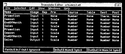
Figure 12.1 NNU translate template for forecasting application.

Please note, however, that sometimes it is better to scale the dependent or output variable in a neural network modeling or forecasting application to a range of 0.1 to 0.9. Driving the output units to their extremes (that is, 0.0 and 1.0 for the standard logistic activation func­tion) requires large connection weights. If the neural network model pre­dicts accurately everywhere but at the extremes, then changing the scaling range could help.

The Neural Network Utility provides a data transformation tool called a Translate Filter. The scaling and transformation of data is specified by some­thing called a Translate template. Figure 12.1 shows the NNU Translate tem­plate we used in this application.

Model and Architecture Selection

As illustrated in Table 4.1 in chapter 4, there are three major types of neural networks that can be used to build time-series forecasting models: back propagation, which is the jack-of-all-trades of neural networks, radial basis function networks, and recurrent back propagation networks. If there is a lot of variability in the data, then radial basis functions might perform best because their fixed center weights allow the network to learn different mappings for different portions of the input space. As the training data moves around, the rest of the radial basis function weights do not degrade. This stability to nonstationary inputs makes radial basis function networks excellent for modeling problems.

Back propagation networks, on the other hand, are susceptible to some­thing called the "herd effect." As the input data moves around the input space, all of the connection weights are adjusted and tend to move to follow the inputs. This behavior occurs when the weights are adjusted after each training pattern is presented, which is the standard technique used. Another

concern when using back propagation for time-series forecasting is that feedforward neural networks have no "memory." If the function being mod­eled has complex dynamics that are dependent on three or four prior states, then all of this information must be presented to the back propaga­tion network at the same time. This technique is called the "sliding window" approach. While it works and has been used for many applications, it does have the drawback that it might require large networks with many input units, which results in long training times.

In some cases, a fully recurrent neural network is required to capture the behavior of complex dynamical systems. However, training recurrent net­works can be extremely time-consuming, making the standard back propa­gation training algorithm seem fast in comparison. In this example, we will try to use the standard back propagation network, and then see if the lim­ited recurrent network provided with NNU performs better.

The number of input and output units is determined by our data rep­resentation and by the number of prior time steps required by the func­tion. In our example, we will use context information and sales data from the current week plus the context information for the next week to pre­dict the next week's sales. This means that we need 13 input units (4 units for promotion, time of year, end-of-month indicator, sales from the current week, 4 units for next week's promotion, next week's time of year, and next week's end-of-month indicator) and a single output unit representing next week's sales.

In addition, we specify one hidden layer with 25 hidden units. As we dis­cussed previously, this initial choice is somewhat arbitrary and selected based on our experience. This experience also tells us that this number might have to be increased or decreased if we have difficulty training the neural network. Do not labor over whether to use 23 or 27 hidden units. While fewer hidden units usually result in better generalization, spending a lot of time searching for the optimal number is often not worth the effort.

Training and Testing the Neural Network

Before we start training the neural network, we first have to decide what level of prediction accuracy is acceptable. The sales forecasting system is going to be used to predict sales two weeks in the future by making two passes through the forecasting model. This gives us some time to either trade with other dealers for inventory, or go to the auto auction to pick up some late-model used cars. An average prediction accuracy of 10% is con­sidered acceptable. In the car business, we aren't ever really in danger of having no cars to sell. The problem is trying to manage the carrying costs of having an overstock on the lot. For the neural network, this translates into an average root mean square (RMS) error of less than 0.10.

We start with a standard back propagation network. Figure 12.2 shows an NNU application module set up for this problem. The Module editor (on the bottom left) shows two Import objects that have our training and testing data. For the training data, we took four and one-half years of weekly sales data. We will test the forecaster with the most recent six months of data. This decision points out one of the problems with time-series forecasting problems. We are using historical data. What if the world has changed in the past six months? How will our neural network ever learn the data? Actually, tliis is a problem even if we used the latest data to train the network. Tomorrow something fundamental to our problem could change (for exam­ple, interest rates go up 2%), which completely blows our model away. The only way we can deal with this is to try to get all of the relevant variables into our model. For example, if sales are sensitive to interest rates, then, by all means, that should be an input variable.

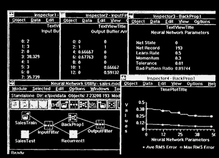
Back to the NNU module again, the Import objects feed their data into the Translate Filter, which preprocesses the data. This data is passed to the neural network, which uses the data in training. The network output is fed into another Translate Filter, which scales the value back up to the number of cars sold.

To monitor the training of our neural network, we open several NNU Inspectors on the module. We open one on the Input Array of the prepro­cessing Translate Filter to see the source data coming from either of our Imports, and we open another one on the Output Array of the Translate Filter to see the preprocessed data going into the Network.

Figure 12.2 NNU module and Inspectors for forecasting application.

On the Network object itself, we open two more Inspectors. One is used to view the key neural network parameters, which in this case are the Net State, the Net Record index, the Learn Rate, the Momentum, the error Tolerance, and the Bad Pattern Ratio. The Net State tells us whether the network is locked or is in training mode. The Net Record index indicates which input record we are processing. Learn Rate, Momentum, and error Tolerance are used to control the learning in the neural network. Finally, the Bad Pattern Ratio is used to monitor the percentage of training patterns that are within our specified Error Tolerance. The second Inspector on the Network object is a time-plot of two error parameters, the average RMS error, and the maxi­mum RMS error.

Because this is a time-series problem, we modify the default Learn Rate and Momentum parameters set by NNU. For Learn Rate we use 0.5 instead of 0.2, and for Momentum we use 0.3 instead of 0.9. Our experience with time-series problems tells us that Momentum can have an adverse impact on training. In some cases it works fine, in others not so well. The behavior of the neural network during training is extremely dependent on the net­work architecture, the data, and the type of function being performed. The initial choices for parameters are not crucial. We typically try a couple of combinations of parameters to see how the network reacts. In general, we want to use the largest learn rate we can to speed up the training. Many de­velopers gradually drop the learn rate as the training progresses to improve predictive accuracy.

We start training the neural network using the NNU Run function. Records are continuously read from the training Import and pass through the con­nected NNU objects. After approximately 100 epochs or complete passes through the training data, the network has already reached an average RMS error of below 0.05. However, the maximum or worst-case prediction error is above 0.20. The prediction errors were coming down nicely but then started to oscillate. This behavior is made obvious by the time-plot Inspec­tor we opened on the network.

As we step through the training data, we examine the input records that are giving the neural network problems. These are the records with the highest prediction errors. It is clear that whenever there is a promotion code of 4 (factory incentives), the network has trouble. This promotion code seems to be a key factor, whether it appears in the current or the up­coming week's context information. Our initial data representation for the promotion field was a one-of-N code. This should give the network enough indication of the "specialness" of the factory code because a single input unit is devoted to representing factory promotions. However, just to make sure this isn't causing problems, we change the NNU Translate Template for the promotion field so that it uses a thermometer code. When the promotion is factory (code value 4) then four inputs are turned on (to 1). This might help the network recognize the significance of the factory promotion more than just having a single one-of-4 inputs turn on with the one-of-N code representation.

We start another training run, and after 75 epochs the average RMS error is 0.06 and the maximum error is now only 0.165. The same network and same parameters were used. So it seems that changing the data represen­tation of the promotion field helped. But sometimes just the difference in the initial random weights can improve (or worsen) the neural network pre­diction accuracy. We lock the network and switch over to the test data, the most recent six months of sales data. The network does well. The average RMS error is 0.068 and worst case is only 0.15. Because the network is con­verging well, we unlock the neural network weights, switch back to the training data, and resume training the network.

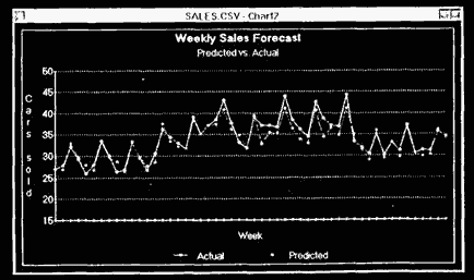
After another 75 epochs, the average RMS error is down to 0.047, while the worst case is still around 0.16 on the training data. This time we open an Inspector on the network output and the desired output and use an NNU time-plot view to see how closely the predictions are tracking the actual sales values. We also logged the actual and predicted values to a comma-de­limited text file. Figure 12.3 is a graph of the actual versus predicted values. While the network is not catching all of the peaks (which look to be occur­ring when the end of month flag is on), it has definitely learned the basic sales curve. The prediction problems at the extremes might be caused by our decision to scale the output value to between 0.0 and 1.0, as we dis­cussed in the data representation section.

Figure 12.3 Graph of predicted versus actual sales.

 

Next we try a limited recurrent back propagation network to see how it per­forms. This type of neural network has a memory and should perform better than regular back propagation on this type of problem. The NNU implemen­tation of the limited recurrent neural networks allows you to specify whether the feedback should come from the first hidden layer of units, or from the out­put layer. In this example, we use the first hidden layer. The effect is that our 25 hidden units are copied back to 25 extra input or context units. This net­work is obviously much larger than the back propagation network.

We train this network using the same data and training parameters as above. After 100 epochs, our network has an average RMS error of 0.049 and a maximum RMS error of 0.143. This is better than the back propagation net­work, but it also took longer to train because of the additional processing units and connection weights. For this time-series forecasting problem at least, the recurrence does not result in any significant improvement in per­formance.

However, this is one of the nice things about using commercial neural net­works tools like NNU. It is very easy to try other neural network models to see if they give better performance than standard back propagation networks.

Deploying and Maintaining the Application

Now that we have an accurate sales forecasting model, the next step is to integrate it into our inventory control system and, to some extent, our staff scheduling system. The inventory control system is an online system that is already automated. However, the staff scheduling system is still done by Charley, the sales manager, who looks at last year's schedule and makes up a new one for this year.

To get a prediction from our neural network, we need to present the same information as during the training process, the prior week's data along with the context information for the next week. In addition, we have to construct the following week's context information and use our first estimate as input to the forecaster a second time. This will give us our forecast for two weeks out.

We have all of this information available, so this is not a problem. The data has to be preprocessed, run through the neural network, and then the out­put has to be scaled back into stock units or number of cars. If we use the Neural Network Utility to deploy this application, we can use the same ap­plication module as we used in the training process. We will have to use the NNU application programming interface (API) to load the application mod­ule and process the source data. Fortunately, this works well on our IBM AS/400 system and can be called by our RPG or COBOL programs.

Maintaining this application will be quite easy. Every month, we can add the last four weeks of sales information to the test data and move four more weeks of data into our training set. Training time takes about ten minutes on a PC, or we can train the neural network on our AS/400 system during our weekend batch processing. As we use the forecasting system, we can see when it is accurate and when it has difficulty. If we notice some new fac­tor that impacts sales, we can start tracking it and add it to our input data at some time in the future. Adding new input variables will require chang­ing the architecture of the neural network and repeating the data mining process we followed in this chapter.

Related Applications and Discussion

Time-series forecasting is a very difficult problem. However, an accurate model can be used very profitably by a business. Mining historical data to discover trends has been one of the most popular uses of neural networks in the past decade (Vemuri and Rogers 1994). Neural networks' ability to model nonlinear functions make them particularly suited to time-series modeling.

Application of time-series prediction include stock price forecasting, electrical power demand forecasting, and sales forecasting. There is a large amount of literature on modeling dynamic systems for control, which is a very-similar problem (Narendra 1992). Forecasting the future state of a sys­tem is also required for building stable controllers for complex systems, such as computer operating systems (Bigus 1993).

In this example, we used a technique known as the "sliding window" to present past information to the neural network so that it could predict ahead, into the future. The function we were modeling, while nonlinear, was relatively simple and required information about one prior state in order to be modeled with reasonable accuracy. Some cases might require five or even ten past states in order for the neural network to capture the dynam­ics. Note that we did not attempt to give the neural network a sequence of weekly sales numbers without providing any context variables. The infor­mation provided by the end-of-month flag and the type of promotion gave the neural network important clues as to the future direction of the sales. Otherwise, the network would have seen unexpected blips at seemingly random times (but we know that it was the end-of-month sales rush, or a factory incentive). It is vitally important to give the neural network what­ever contextual information is available. Predicting the future is hard enough, even with all of the available information.

Summary

In this chapter, we created a neural network forecasting tool to predict weekly sales at an automobile dealer. We provided information on the cur­rent week's sales and context information, such as planned promotions, for the future week. We computed time of year and time of month information

from the date and tried several data representations in our application. The IBM Neural Network Utility was used to perform the data pre- and postpro­cessing and to train and test our neural networks. Our forecasting model was able to predict with an average accuracy of greater than 95%. We iden­tified that factory promotions caused extreme fluctuations in the weekly sales figures.

Mining historical data to build time-series forecasters is one way of learn­ing from past experience. Neural networks can discover hidden relation­ships in temporal data and can be used to develop powerful business applications.