Source: http://citeseer.ist.psu.edu/cache/papers/cs/733/http:zSzzSzwww.brunel.ac.ukzSz~cspgsskzSzdocumentszSztech-reportszSzCNES-96-04.pdf/diagnosis-of-oral-cancer.pdf

Simon Kent

Diagnosis of Oral Cancer using Genetic Programming

Abstract

Genetic Programming is a relatively new technique for the automatic discovery of computer programs which offer solutions to complex problems. It is being applied to an ever increasing number of application areas with good results.

This report presents some introductory work on a classification problem. The Genetic Programming technique is used to evolve programs which are able to diagnose oral cancer and pre-cancer in a sample of patients. Real data on the habits and lifestyles of patients is used to train and test the system.

Despite inconsistencies in the input data, and a low proportion of positive samples, the evolved programs make accurate predictions and compete favourably with a previous neural network implementation of this problem.

1 Introduction

Genetic Programming (GP) uses evolutionary principles borrowed from nature, and applies them in a computer to generate programs to solve complex problems. The technique is still very much in its infancy, its birth being attributed to Koza (1989), however, it is rapidly finding a wide variety of application areas. This report discusses its use in generating programs capable of diagnosing oral cancer.

The problem presented here is one of classification. This is a task which has been successfully tackled using other techniques such as neural networks (NN). The data used in this project has previously been used by Elliott (1993) to solve this same diagnosis problem using neural networks. Elliott’s work provides a useful benchmark with which to compare the results from this GP project.

2 Genetic Programming

Genetic Programming uses the Darwinian principle of natural selection to produce solutions to problems. Animals and plants which have evolved in nature represent extremely complex solutions to the problem which they face of surviving in the environment in which they live. It would be extremely valuable if computers could provide solutions with even a fraction of the complexity of a simple mammal. Using GP, it may be possible to apply computer technology to problems which are too complex to solve by a human programmer using conventional methods in computer science.

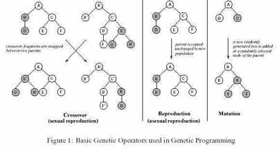
In biological evolution, individuals are created by either sexual or asexual reproduction, each individual taking on some of the characteristics of its parents. The most successful individuals will reproduce more than less fit individuals. In this way, the characteristics which make the individual successful will be passed on to successive generations. The fitter the individual, the greater the likelihood that it will reproduce. Therefore, ‘good’ genetic material is transmitted through successive generations. This is how mankind and other mammals have reached their present, advanced state.

In GP, the individuals which take part in evolution are computer programs which pose a solution to a given problem. Computer programs can be represented as trees, and the production of successive generations is achieved by applying genetic operators, as shown in Figure 1. These mimic the mating process.

Evolution is captured in a repetitive computational process. An initial population is generated randomly as a starting point for the process. Each individual is executed to measure its fitness or ability to solve the problem for which it is intended. A new population is then generated from the previous generation, using the genetic operators. The probability that a particular individual participating in the generation of an individual in the new generation, increases with its fitness. This process of fitness evaluation and evolution is repeatedly applied until a solution is found or a timeout occurs.

The Genetic Programming technique is only described very briefly in this report. A much more in depth coverage of GP can be gathered from Koza (1993).

3 Source Data

The data used in this project was originally collected at the Eastman Dental Institute in London. It was collected from questionnaires given to patients prior to a screening process. Each questionnaire also contained data from two people performing diagnoses of the patients’ conditions. One diagnosis was made by a non-specialist screener, while the other was made by a specialist. The specialist was able to carry out a diagnosis using diagnostic aids such as biopsy. There were a total of 2027 records available, however some of these were discarded as described below in section 3.3.

3.1 Questionnaire Data

The questions asked of the patients were multiple choice questions, restricting the subject’s answers to discrete bands. For example, for question 5 below, the patient was given a choice of never; not for over ten years; within the last ten years; current user. The questions contained on the questionnaire were as follows:

1. Sex
2. Date of Birth
3. Date of screening
4. Department in which screened
5. Smoked or chewed
6. For how long smoked or chewed
7. Smoked filtered cigarettes
8. Smoked unfiltered cigarettes
9. Smoked cigars
10. Number smoked per day
11. Smoked rollups
12. Smoked a pipe
13. Chewed tobacco
14. Chewed betelnut
15. Ounces smoked/chewed per day
16. Drink alcohol
17. Drink beer
18. Drink wine
19. Drink fortified wine
20. Drink spirits
21. Units drunk per week
22. Time of last visit to dentist
23. Name of screener
24. Screener Result
25. Location in mouth of problem (according to screener)
26. Type of problem (according to screener)
27. Specialist Result
28. Location in mouth of problem (according to specialist)
29. Type of problem (according to specialist)

3.2 Data Representation

The questionnaire data was not in a suitable form for direct use by the GP diagnosis software as it was collected in a Paradox database. It also contained superfluous data, for example ‘name of screener’ which would be irrelevant for performing a correct diagnosis.

The data was exported from the Paradox database as delimited text, and converted to a 13-bit bit-field for each record. Each bit represents the truth value of one of thirteen predicates about the patient. The questions or predicates are based on those used by Elliott (1993) in his MSc project. His questions were developed jointly by himself and Joanna Julien who was the specialist who provided the human diagnoses of the dental patients.

The thirteen predicates are as follows:

1. Sex is female (i.e. 0=Male, 1=Female)

2. Age >40

3. Age > 55

4. Age >70

5. Age >85

6. Have been smoking within last 10 years

7. Currently smoke >=20 cigarettes per day

8. Have been smoking for >=20 years

9. Beer and/or wine drinker

10. Fortified wine and/or spirit drinker

11. Drink excess units (i.e. Male >21, Female >14

12. Not visited dentist in last 12 months

13. Positive specialist diagnosis

3.3 correctness

No checks were made to confirm the correctness of the answers given in the questionnaires. Relying only on the honesty of the patient subjects inevitably led to innacuracies in the data. It is a difficult task, and outside the scope of this report, to carry out a detailed analysis of the data to find inconsistencies.

Some checking was performed on the data. Firstly a quick visual check was performed to identify clearly incorrect data such as patient ages of 0.17 or even -0.01.

After the data had been converted to bit-fields (see section 4), it was passed through a program which checked for inconsistencies. That is where identical records of input bit-fields map to conflicting expert diagnoses. These could arise as a result of incorrect data in the original questionnaires, or it could be attributed to the lost information caused by the bit-field conversion. A bit-field provides a lower resolution representation of the characteristics of the patient than does the original questionnaire data. For example, the bit-fields do not contain any information about the type of tobacco used, but the original questionnaire data does.

The data was found to include 37 groups of individuals which contained inconsistencies. Most of these groups were of between 2 and 4 records in size. In total, 110 individuals were affected. Two of these groups affected a particularly large number of individuals; 10 and 11 respectively. These two offending groups were removed from the data set. The other smaller inconsistency groups were left in the data, as it was felt that these represented noise which would always naturally arise in such data.

As a result of the checks made on the data, 31 individuals were removed from the data leaving a set of 1996 individuals, of which 54 were positive diagnoses, and 1440 were negative diagnoses. These were split into a training set and a test set. The training set contained 1483 records (43 positive, 1440 negative) and the test set contained 513 records (11 positive, 502 negative). The training set was left with 29 groups of inconsistencies, and the test set with 8.

4 GP Representation Scheme

Genetic Programming requires a representation scheme with which it can express a solution to the problem which it is trying to solve. Solutions to GP problems are expressed as programs or trees. These trees are constructed from functions which are the internal nodes of the trees, and terminals which form the leaves of the trees.

4.1 Terminal Set

The terminal set for this problem consists of the thirteen bit-fields which represent a particular patient’s lifestyle and habits. That is, a leaf value will represent a truth value for one of the thirteen predicates in 3.2.

4.2 Function Set

The function set consists of three logical operators: AND, OR, and NOT. A solution to the problem will therefore be a logical expression using patient attributes as variables.

5 Fitness Measure

Genetic Programming generates candidate solutions to the problem being solved. It is necessary to have a method of measuring how effectively a program solves the problem. This is known as the fitness measure. It is important that this measure accurately assesses the performance of a program. A poor fitness measure will encourage the GP system to solve a different problem to that which is intended.

5.1 Percentage Correct and Mean Square Error

For this oral cancer problem, a program is evaluated against each of the patient data records in the training set. Two methods considered were:

• Mean square error of patient diagnosis
• Proportion of patients correctly diagnosed

For this problem, these two methods are equivalent, as one of them is equal to 1.0 minus the other. Therefore they unfortunately suffer from the same problem in that some of the GP tree solutions which they suggest are highly fit, are not those which will contribute to the evolution of optimum individuals in the long run. As an example, ms-error for this problem is defined as:

In theory this may seem to present a suitable fitness measure, however in practice it causes a problem which degrades the performance of the evolutionary process. The problem is caused by certain individuals which inevitably appear in the population. These are those which output a single truth value regardless of the input variables. A simple example of such an individual is shown in figure 3. This contradictory tree will always output a false truth value.

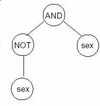
Figure 3: A contradictory tree

If a contradictory individual is evaluated against the training set discussed in section 3.3, the ms-error will be calculated as 0.029. These contradictory individuals have much better fitnesses than other individuals, so their genetic material quickly dominates the population, and causes rapid convergence to a sub-optimal solution, rather than encouraging the gradual evolution to an optimal solution. Such solutions will provide a high overall percentage of correct diagnoses, however these are all negative diagnoses which dominate the input data, while none of the positive cases will ever be recognised.

Use of the percentage of patients correctly diagnosed as the fitness measure gives rise to the same problem. A contradictory individual which is very unintelligent, will be able to correctly diagnose 97% of the individuals (the negative ones). Other individuals may contain important genetic material which could contribute during a later generation to an effective solution, but these are oppressed by the apparently superior contradictory individuals. This problem emphasises the need for a more suitable fitness measure.

5.2 Shifted Fitness

The fitness problem was addressed by using a scheme as shown in figure 4. Here, the contradictory individuals which previously caused problems are centred at 0.5, thus relatively reducing their fitness. The optimum target is valued at 1.0 and the worst case is at 0.0, where the individual incorrectly diagnoses all patients. This method rewards for correct diagnoses and punishes for incorrect diagnoses more effectively than the previous two methods. This shifted fitness method is the one which was used in all diagnosis experiments.

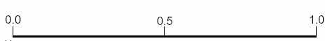
Figure 4: A ‘shifted’ fitness scheme

population size	500
maximum depth of individuals in initial population	6
maximum depth of individuals in evolved population	17
generative method	ramped half-and-half
Probability of function node	0.80
Probability of terminal node	0.20
crossover probability	0.90
reproduction probability	0.10
mutation probability	0
probability of choosing function node for crossover	0.90
selection method	tournament

Table 1: GP Parameters for the Oral Cancer Diagnosis Problem.

6 Genetic Programming Parameters

The basic GP process can be tuned using a number of parameters. Table 1 lists the values of the main parameters used in the runs for this report.

6.1 Population Size

The population size is the number of genetic programs in each generation of the genetic programming process. Typically, a more difficult problem would employ a larger population.

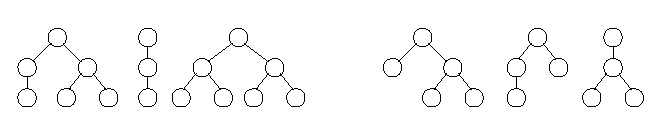
Figure 5: Full and Grow generated trees

6.2 Population Generation

Limits are set to prevent the sizes of the data structures becoming too large. One limit is set on the depth of the programs in the initial, randomly generated population, and a second is set on depth of those programs which are generated as a result of a genetic operation such as reproduction, crossover or mutation (see 2).

The ramped half and half method of population generation attempts to produce a varied first generation with many different types of trees. Half of the generated population will contain full trees which have all their leaf nodes at the same depth. In these trees, a function node is generated at each level until the deepest permissible level is reached, at which point a terminal node is generated. Example full and grow trees are shown in figure 5.

The other half of the population contains grow trees. The shape of grow trees is determined probabilistically using the probability of function and terminal node parameters. When creating each node using the grow method, a decision is made as to which type of node; function or terminal; to generate. In this case, 80% of the nodes will be function nodes, and 20% will be terminal nodes. As with full trees, when the maximum depth is reached, the generation of a terminal node is forced.

During the generation of each half of the population, the maximum depth of the individual programs is incremented from 2 to the maximum depth (6 in this case), to ensure the widest possible variety of individuals in terms of shape and size. It is worth noting that to further ensure variety in the initial population, a check is performed to ensure that each individual is unique.

6.3 Evolution

The probability of crossover, reproduction and mutation represent the likelihood of each of the respective genetic operations being used in the evolution of one generation to the next generation. In this case, 90% of the time crossover is used, 10% of the time reproduction is used, and mutation is never used.

The parameter controlling the probability of choosing a function node for crossover is set high to ensure that most of the time when crossover is applied, the crossover fragments are small sub-trees rather than individual leaf nodes. This encourages the generation of larger structures, rather than just swapping single nodes.

When performing evolution, individuals must be chosen from a population to participate in a genetic operation. Tournament selection firstly involves randomly choosing two individuals from the parent population. The member of the pair with the highest fitness wins, and hence is allowed to participate in a genetic operation. This method attempts to mimic the type of competition between animals for the right to mate with each other.

7 Results

It was necessary to run the GP system several times with different initial populations. It was felt to be important to present an arbitrary sequence of runs. There has been no filtering out of particularly poor runs. The results are intended to demonstrate the consistency with which the GP system can perform highly for this problem.

A graph of the results of 13 runs of the system is shown in figure 6 which shows the performance of the best of run individual against the training set. A corresponding graph in figure 7 shows the performance against the test set. For each run, three bars are present. The first represents the the percentage of correct overall diagnoses, the second shows the percentage of correct positive diagnoses, and the third shows the percentage of correct negative diagnoses.

The solutions we are interested in are those which are able to correctly diagnose a high number of positive and negative cases. We are also interested in solutions which are good at generalising, that is where there is a close correlation between the results in the training set and test set. In a commercial application, a good solution would be expected to perform well when presented with a wide range of test sets. A comparison between the training and test set results is shown in figure 8.

On this basis, runs 3, 8 and 10 both offer good solutions, but the best solutions appear in run 6 and 13. The best solution from run 6 correctly predicts 63% of the positive diagnoses and 71% of the negative diagnoses in the training set, whilst in the test set it correctly diagnoses 64% of the positive cases, and 65% of the negative cases. Run 13 correctly predicts 63% of positive cases and 69% of negative cases in the training set, whilst in the test set it predicts 64% of positive cases and 61% of negative cases.

The best solution from run 6 is a 96 node program, which was of depth 12, and from run 13 is a 75 node program of depth 16. Both these individuals can be found in the appendix.

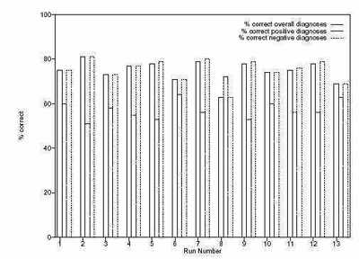
Figure 6: Results of 13 runs against training set

8 Conclusions

The results have clearly demonstrated that genetic programming can be used effectively for the diagnosis of oral cancer from patient questionnaire data.

The results are particularly pleasing in light of the problem of inconsistencies in the source data. This indicates that such a GP system would be of practical use in a real-world diagnosis application where such noise would be inevitable.

A further point which could have inhibited the performance of the system is that there were relatively few positive examples from which the system could learn. In fact only 2.7% of the individuals in the source data were positively diagnosed by the dental expert.

Elliott’s (1993) work reports that his system was able to correctly diagnose 73% of positive cases, and 71% of negative cases in his test set. The results from the GP system therefore compare favourably with his results. It must be noted that a comparison between the methods is difficult as the Elliott’s exact results are not known, and the test and training sets used by the two systems differ.

% correct Assuming that the GP system has a similar ability to diagnose oral cancer as a neural network system, it still offers a major advantage. The best solution which it produces can be examined by a human, who will be able to understand the logic behind the diagnostic decision of the software. A similar solution from a neural network will simply be a mass of weights, the meaning of which will be much more difficult to ascertain. In GP, the representation scheme is application specific.

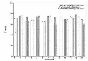
Figure 7: Results of 13 runs against test set

9 FurtherWork

9.1 Improved comparison with Neural Networks

The vague comparison between the Genetic Programming system and a Neural Networks solution was given in section 8. Ciaran Elliott, an MSc student at Brunel is undertaking a project (Elliott, 1996) to produce a NN diagnostic tool using exactly the same data as was used in this project. Given full access to his methods and results, it is hoped that a much more reliable comparison can be made in the future.

9.2 Medical Diagnosis Applications

Genetic Programming has been shown to effectively diagnose oral cancer. There does not appear to be any reason why this should not be extended to the diagnosis of other conditions and diseases in the medical world.

In this project the variables contributing to a diagnosis were known in advance. It may be possible to extend a diagnosis system to take a large number of general patient attributes, gathered for example at a medical, and use GP to determine which of these attributes are relevant in the diagnosis of a particular ailment.

A rapid diagnostic system which can adapt over time would be invaluable for rapid screening of patients for a large number of problems very quickly and without the high cost of existing screening techniques.

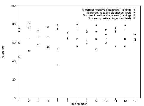
Figure 8: Comparison between training and test sets of 13 runs

Acknowledgements

I would like to thank the Eastman Dental Institute for providing the data for this project, and Dr Dimitris Dracopolous for his support and advice. This work was partly supported by EPSRC award number 95700741.

References

Elliott, A. (1993). The use of neural networks in medical statistical analysis, Master’s thesis, Eastman Dental
Institute.
Elliott, C. (1996). The use of inductive logic programming and data mining techniques to identify people at
risk of oral cancer and precancer, Master’s thesis, Brunel University.
Koza, J. R. (1989). Hierachical genetic algorithms operating on populations of computer programs,
Proceedings of the 11th International Joint Conference on Artificial Intelligence .
Koza, J. R. (1993). Genetic Programming: on the Programming of Computers by means of Natural Selection,