IE (I) Journal-ET, Vol 84, January 2004
Image Classification Based on Textural Features using Artificial Neural Network (ANN)
Prof S K Shah, Fellow
V Gandhi, Non-member
Department of Electrical Engineering, M S University of Baroda, Kalabhavan, Baroda
Image classification plays an important part in the fields of Remote sensing, Image analysis and Pattern recognition. Digital image classification is the process of sorting all the pixels in an image into a finite number of individual classes. The conventional statistical approaches for land cover classification use only the gray values. However, they lead to misclassification due to strictly convex boundaries. Textural features can be included for better classification but are inconvenient for conventional methods. Artificial neural networks can handle non-convex decisions. The uses of textural features help to resolve misclassification. This paper describes the design and development of a hierarchical network by incorporating textural features. The effect of inclusion of textual features on classification is also studied.
Keywords: Gray values; Neural classifier; Supervised classifier; Textural features.
IMAGE CLASSIFICATION
Digital image consists of discrete picture elements called pixels which are associated with a digital number represented as DN that depicts the average radiance of relatively small area within a scene. The range of DN values is normally 0 to 255. Digital image processing is a collection of techniques for the manipulation of digital images by computers.
Classification generally comprises four steps:
- Pre-processing - eg, atmospheric correction, noise suppression, and finding the band ratio, principal component analysis, etc.
- Training - selection of the particular feature which best describes the pattern.
- Decision - choice of suitable method for comparing the image patterns with the target patterns.
- Assessing the accuracy of the classification.
The informational data are classified into supervised and unsupervised systems.
ARTIFICIAL NEURAL NETWORK (ANN)
ANN according to Haykin is a massively parallel distributed processor that has a natural propensity for storing experiential knowledge and making it available for use. ANNs can provide suitable solutions for problems, which are generally characterized by non-linearities, high dimensionality noisy, complex, imprecise, imperfect or error prone sensor data, and lack of a clearly stated mathematical solution or algorithm. A key benefit of neural networks is that a model of the system or subject can be built just from the data.
Supervised learning is a process of training a neural network with examples of the task to learn, ie, learning with a teacher.
Unsupervised learning is a process when the network is able to discover statistical regularities in its input space and automatically develops different modes of behaviour to represent different classes of inputs.
NETWORK ARCHITECTURE
Texture is characterized by the spatial distribution of gray levels in a neighbourhood. Since, texture shows its characteristics by both pixel co-ordinates and pixel values, there are many approaches used for texture classification. The gray-level co-occurrence matrix seems to be a well-known statistical technique for feature extraction.
In texture classification the goal is to assign an unknown sample image to one of a set of known texture classes.
Textural features can be either scalar numbers, discrete histograms or empirical distributions. They characterize the textural properties of the images, such as spatial structure, contrast, roughness, orientation, etc and have some correlation with the desired output.
There are fourteen textural features. The design considers four features namely angular second moment (ASM), contrast, correlation, variance. However, it can be extended by inclusion of all features. The system architecture of the combined approach using both gray values and textural features is shown in Figure 1.
Architecture using Gray Values Only
The authors have considered a four layer ANN comprising three inputs, seven first layer hidden nodes, eleven second layer hidden nodes and five output nodes. Figure 2 shows the architecture of this network. Training of the network is done using standard BKP.
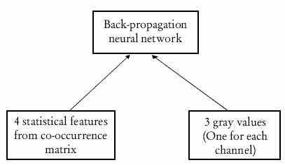
Figure 1 System architecture of combined approach
Using Gray Values and Textural Features
Combining both gray values and textural features form a four layer artificial neural network comprising seven inputs, eleven first layer hidden nodes, fifteen second layer hidden nodes and five output nodes. Figure 3 shows the architecture of this network.

Figure 2 Architecture of NN with only gray values
The number of bands and classes determine the number of input and the output nodes, respectively.
ALGORITHM
Feature Extraction
Texture and tone bear an inextricable relationship to one another. Tone and texture are always present in an image, although at times one property can dominate the other. For example, when a small area patch of an image has little variation of features of discrete gray tone, then tone is the dominant property. Important property of tone texture is the spatial pattern of resolution cells composing each discrete tonal feature. When there is no spatial pattern and the gray tone variation between features is wide, a fine textural image results.
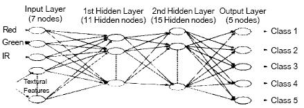
Figure 3 Architecture on NN with combined gray value and textural features
Texture is one of the most important defining characteristics of an image. It is characterized by the spatial distribution of gray levels in a neighbourhood. In order to capture the spatial dependence of gray-level values, which contribute to the perception of texture, a two dimensional dependence, texture analysis matrix is considered. Since, texture shows its characteristics by both pixel and pixel values, there are many approaches used for texture classification. The gray-tone cooccurrence matrix is used for feature extraction. It is a two dimensional matrix of joint probabilities Pd, r (i, j) between pairs of pixels, separated by a distance, d in a given direction r1.
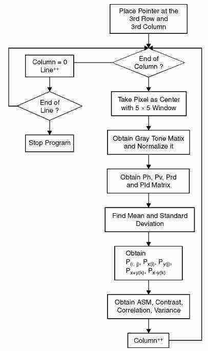
- For finding textural features for every pixel in the image every pixel is considered as a centre and followed by a 5 ? 5 window about that centre pixel.
- The gray-one matrix for that particular window is calculated and normalized.
- The gray level co-occurrence matrix namely, Ph, Pv, Prd and Pld for each pixel is then obtained. Here, Ph, Pv, Prd and Pld are respectively the 0o, 90o, 45o and 135o nearest neighbours to a particular resolution cell.
- Standard deviation and mean are now obtained for each of these matrices and are used later to calculate the textural features.
- Now the particular entry in a normalized gray tone spatial dependence matrix is calculated for further reference, ie, P (i, j), Px (i), Py ( j ), Px + y (k) and Px - y (k).
- Using the formulas of the textural features, the angular second moment, contrast, correlation and variance are calculated (Appendix A).
Training the Combined Network using BKP
The following assumes the sigmoid function f (x):

The popular BKP algorithm1,2 is implemented using following steps:
Step 1: Initialize weights to small random values.
Step 2: Feed input vectors X0, X1, . . . . . . . . . . , X6 through the network and compute the weighting sum coming into the unit and then apply the sigmoid function. Also, set all desired outputs d0, d1 . . . . . d5 typically to zero except for that corresponding to the class the input is from.
Step 3: Calculate error term for each output unit as

where dj is the desired output of node j and yj is the actual output.
Step 4: Calculate the error term of each of the hidden units as

where k is over all nodes in the layers above node j and j is an internal hidden node.
Step 5: Add the weight deltas to each of

All the steps excepting step 1 are repeated till the error is within reasonable limits and then the adjusted weights are stored for reference to the Recognition Algorithm.
Illustration
As an application the image Figure 4(a) is considered from which a portion Figure 4(b) has been extracted which needs to be classified into five different classes considering both gray values and textural features. The pixels selected for training have been taken from the whole image except the portion, which is extracted for classification. For evaluating the accuracy of the classification, pixels of known class have been used.
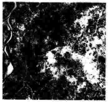
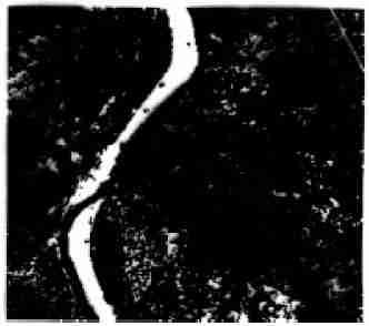
Figure 4(a) Original image Figure 4(b) Segmented image


Figure 5(a) [Left] with only gray values Figure 5(b) [Right] : including textural features
TRAINING PIXELS:
| Land Cover Type | No of Pixels | |
| Barren (B) | Class 1 | 20 |
| Sand (S) | Class 2 | 20 |
| Urban (U) | Class 3 | 20 |
| Vagetation (V) | Class 4 | 20 |
| Water (W) | Class 5 | 20 |
| Total | 100 |
| Land Cover Type | |||||||
| Classes | B | S | U | V | W | Overall | Average |
| Class 1 | 19 | 0 | 1 | 0 | 0 | 95% | |
| Class 2 | 0 | 20 | 0 | 0 | 0 | 100% | |
| Class 3 | 3 | 0 | 17 | 0 | 0 | 85% | 91% |
| Class 4 | 0 | 0 | 0 | 20 | 0 | 100% | |
| Class 5 | 1 | 0 | 0 | 4 | 15 | 75% | |
| Total | 23 | 20 | 18 | 24 | 15 | ||
With Gray Values Only
| Land Cover Type | |||||||
| Classes | B | S | U | V | W | Overall | Average |
| Class 1 | 20 | 0 | 0 | 0 | 0 | 100% | |
| Class 2 | 0 | 16 | 0 | 0 | 4 | 80% | |
| Class 3 | 0 | 10 | 0 | 0 | 10 | 50% | 46% |
| Class 4 | 20 | 0 | 0 | 0 | 0 | 0% | |
| Class 5 | 20 | 0 | 0 | 0 | 0 | 0% | |
| Total | 60 | 26 | 0 | 0 | 14 | ||

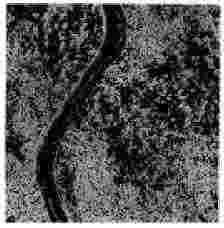
6(a) CLASS 1 : BARREN 6(d) CLASS 1 : BARREN
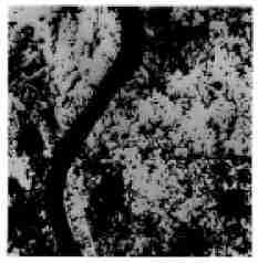
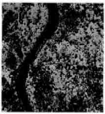
6(b) CLASS 4 : VEGETATION 6(e) CLASS 4 : VEGETATION

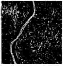
6(c) CLASS 5 : WATER 6(f) CLASS 5 : WATER
