Source: www.pmarneffei.hku.hk/mbetoolbox/matlab_doc/toolbox/powersys/synchronousmachine.html

Synchronous Machine

      Purpose: Model the dynamics of a three-phase round rotor or salient-pole synchronous machine

Description

      The Synchronous Machine block operates in generating or motoring modes. The operating mode is dictated by the sign of the mechanical power (positive for generating, negative for motoring). The electrical part of the machine is represented by a sixth-order state-space model and the mechanical part is the same as in the Simplified Synchronous Machine block.
      The model takes into account the dynamics of the stator, field, and damper windings. The equivalent circuit of the model is represented in the rotor reference frame (qd frame). All rotor parameters and electrical quantities are viewed from the stator. They are identified by primed variables. The subscripts used are defined as follows:
      • d,q: d and q axis quantity
      • R,s: Rotor and stator quantity
      • l,m: Leakage and magnetizing inductance
      • f,k: Field and damper winding quantity
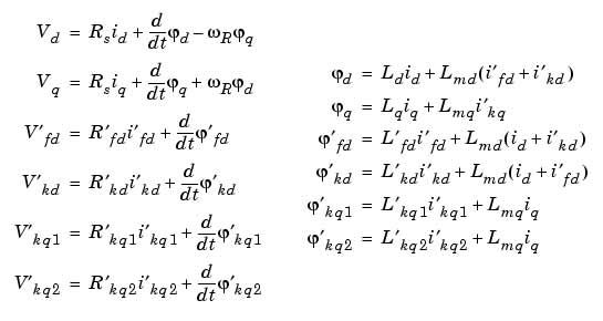
      The electrical model of the machine is

      with the following equations:

Dialog Box and Parameters

       In the powerlib library you can choose among three Synchronous Machine blocks to specify the parameters of the model.

Fundamental Parameters in SI Units

Rotor type

      Specifies rotor type: salient-pole or round (cylindrical). This choice affects the number of rotor circuits in the q-axis (damper windings).

Nominal

       The total three-phase apparent power Pn (VA), rms line-to-line voltage Vn (V), frequency fn (Hz), and field current ifn (A).
       The nominal field current is the current that produces nominal terminal voltage under no-load conditions. This model was developed with all quantities viewed from the stator. The nominal field current makes it possible to compute the transformation ratio of the machine, which allows you to apply the field voltage viewed from the rotor, as in real life. This also allows the field current, which is a variable in the output vector of the model, to be viewed from the rotor. If the value of the nominal field current is not known, you must enter 0. Since the transformation ratio cannot be determined in this case, you have to apply the field voltage as viewed from the stator and the field current in the output vector is also viewed from the stator.

Stator

       The resistance Rs (), leakage inductance Lls (H), and d-axis and q-axis magnetizing inductances Lmd (H) and Lmq (H).

Field

      Field The field resistance Rf' () and leakage inductance Llfd' (H), both referred to the stator.

Dampers

      Dampers The d-axis resistance Rkd' () and leakage inductance Llkd' (H), the q-axis resistance Rkq1' () and leakage inductance Llkq1' (H), and (if round rotor only) the q-axis resistance Rkq2' () and leakage inductance Llkq2' (H). All these values are referred to the stator.

Mechanical

       The inertia coefficient J (kg.m2), damping coefficient D (N.m.s./rad), and number of pole pairs p.

Initial conditions

       The initial speed deviation dw (% of nominal speed), electrical angle of the rotor Oe (deg), line current magnitudes ia, ib, ic (A) and phase angles pha, phb, phc (deg), and the initial field voltage Vf (V). You can specify the initial field voltage in one of two ways. If you know the nominal field current (first line, last parameter) enter in the dialog box the initial field voltage in volts DC referred to the rotor. Otherwise, enter a 0 as nominal field current, as explained earlier, and specify the initial field voltage in volts DC referred to the stator. You can easily determine the nominal field voltage viewed from the stator by selecting the Display Vfd which produces a nominal Vt check box at the bottom of the dialog box.

Simulate saturation

      Simulate saturation Specifies whether magnetic saturation of rotor and stator iron is to be simulated or not.

Saturation

      The no-load saturation curve parameters. Magnetic saturation of stator and rotor iron is modeled by a nonlinear function, in this case a polynomial, using points on the no-load saturation curve. You must enter a 2-by-n matrix, where n is the number of points taken from the saturation curve. The first row of this matrix contains the values of field currents, while the second row contains values of corresponding terminal voltages.

      The first point (first column of the matrix) must correspond to the point where the effect of saturation begins. You must select the Simulate saturation check box to simulate saturation. This check box allows you to enter the matrix of parameters for simulating the saturation. If you do not want to model saturation in your simulation, simply do not select the Simulate saturation check box. In this case the relationship between ifd and Vt obtained is linear (no saturation).

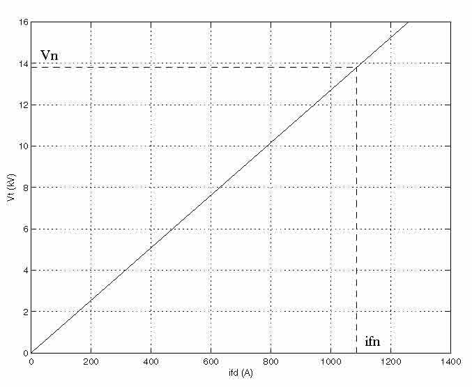
      As an example, without saturation, a typical curve might be as shown below. Here ifn is 1087 A and Vn is 13800 V rms line-to-line, which is also 11268 V peak line-to-neutral.

       When saturation is modeled, a polynomial is fitted to the curve corresponding to the matrix of points you enter. The more points you enter, the better the fit to the original curve.

       The next figure illustrates this graphically (the diamonds are the actual points entered in the dialog box).

In this particular case, the following values were used:
       • ifn = 1087 A
       • ifd= [695.64, 774.7, 917.5, 1001.6, 1082.2, 1175.9, 1293.6, 1430.2, 1583.7] A
       • Vt = [9660,10623,12243,13063,13757,14437,15180, 15890, 16567] В

[Библиотека]