Automatic Speech Recognition Using Hidden Markov Models

Source: http://www.caip.rutgers.edu/multimedia/speech-recognition/thesis.pdf

As the speed of computers gets faster and the size of speech corpora becomes larger, more computationally intensive statistical pattern recognition algorithms which require a large amount of training data are becoming popular for automatic speech recognition. A hidden Markov model (HMM) [81] is a stochastic method, into which some temporal information can be incorporated. In this chapter, the fundamentals of speech recognition algorithms that make use of HMM are described. Figure 2.1 shows a block diagram of a typical speech recognition system. First, feature vectors are extracted from a speech

Структура распознавателя речи

waveform. Then, the most likely word sequence for the given speech feature vectors is found using two types of knowledge sources, i.e., acoustic knowledge and linguistic knowledge. The HMM is used to capture the acoustic features of speech sound and the stochastic language model is used to represent linguistic knowledge. In this chapter, each component of the block diagram is explained in detail.

2.1 Feature Extraction

For automatic speech recognition by computers, feature vectors are extracted from speech waveforms. A feature vector is usually computed from a window of speech signals (20 ..30 ms) in every short time interval (about 10 ms). An utterance is represented as a sequence of these feature vectors. A cepstrum [14][76] is a widely used feature vector for speech recognition. The cepstrum is defined as an inverse Fourier transformation of a logarithmic short-time spectrum. Lower order cepstral coefficients represent the vocal tract impulse response. In an effort to take auditory characteristics into consideration, the weighted averages of spectral values on logarithmic frequency scale are used instead of magnitude spectrum, producing mel-frequency cepstral coefficients (MFCC) [17]. The time derivatives of the MFCC are usually appended to capture the dynamics of speech. See Section 5.2.1 for the detail of feature extraction procedure. Figures 2.2 (b) and (c) are the spectrogram and MFCC extracted from the example utterance.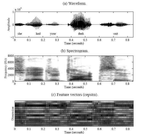

Представление речи

Figure 2.2: An example of speech waveform, spectrogram, and feature vectors.

One popular technique for robust speech recognition, which is applied to cepstral coefficients, is cepstral mean normalization (CMN) [2][25]. Since convolutional distortions such as reverberation and different microphones become additive offsets after taking the logarithm, subtracting the noise component from distorted speech will provide the clean speech component. However, estimating convolutional noise from distorted speech is not an easy task. The CMN approximates the convolutional noise component with the mean of cepstra, assuming that the average of the linear speech spectra is equal to 1, which is obviously not true. The mean vector of each utterance is computed and subtracted from the speech vectors. It has been observed that the CMN produces robust features for the convolutional noise case (see Section 5.3.3). Although the CMN is simple and fast, its effectiveness is limited to the convolutional noise because it removes the spectral tilt caused by the convolutional noise. Also, estimating the mean vector is not reliable when an utterance is too short.

2.2 Hidden Markov Models

Speech recognition can be considered as a pattern recognition problem. If the distribution of speech data is known, a Bayesian classifier,

Формула

finds the most probable utterance U(word sequence), for the given feature vectors X (observation sequence). Bayesian classifiers are optimal in a sense that the probability of error is minimum [19][24]. An HMM [81] can be considered as a special case of the Bayesian classifier. In this section, how speech is represented by an HMM is discussed.

2.2.1 Acoustic Modeling

One of the distinguishing characteristics of speech is that it is dynamic. Even within a small segment such as a phone , the speech sound changes gradually. The beginning of a phone is affected by the previous phones, the middle portion of the phone is generally stable, and the end is affected by the following phones. The temporal information of speech feature vectors plays an important role in recognition process. In order to capture the dynamic characteristics of speech within the framework of the Bayesian classifier, certain temporal restrictions should be imposed. A 3-state left-to-right HMM is usually used to represent a phone. Figure 2.3 shows an example of such an HMM, where Aij represents a state transition probability from the state I to the state j, and bi(х) is the observation probability of the feature vector Х given the state I. Each state in an HMM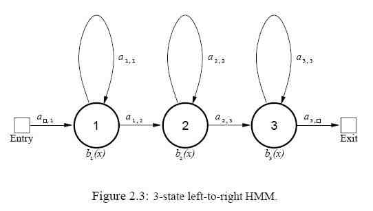

Формула

models the distribution of a sound in a phone. The phone HMM in Figure 2.3 consists of 3 consecutive distributions. A word HMM can be constructed as a concatenation of phone HMM’s. A sentence HMM can be made by connecting word HMM’s. The probability of speech feature vectors generated from an HMM is computed using the transition probabilities between states and the observation probabilities of feature vectors given states. For example, consider an observation sequence consisting of seven vectors;

Формула

denotes a feature vector at time tin the sequence. Suppose that the first two vectors belong to the first state, the next three vectors belong to the second state, and the rest belong to the last state. The probability of the observation sequence X and this state assignment S, given the utterance HMM U, can be computed as follows;

Формула

where Aij is the state transition probability, and Bi(x(t)) is the observation probability of the feature vector x(t) given the state I. To compute the probability of the observation sequence X given the HMM U, all conditional probabilities of X and S given U have to be summed over all possible state/vector assignments (also called state/frame alignment);

Формула

where S* is all possible state sequences. This summation takes O(|s*||x|) time in general, where |s*| is the number of states in an HMM and |X| is the number of feature vectors. There exists a more efficient algorithm that takes polynomial time, which will be discussed in Section 2.3.

2.2.2 Sub-word Modeling

In large vocabulary speech recognition (LVCSR), it is difficult to reliably estimate the parameters of all the word HMM’s in the vocabulary because most of the words do not occur frequently enough in training data. Furthermore, some of vocabulary words may not even be seen in the training data, which degrades recognition accuracy [52]. On the other hand, the number of sub-word units such as phones are usually smaller than the number of words. Most languages have about 50 phones. There are more data per phone model than per word model, and all phones occur fairly often in a reasonable size training data [55]. A monophone HMM models one phone. It is a context-independent unit in the sense that it does not distinguish its neighboring phonetic context. In fluently spoken speech, however, a phone is strongly affected by its neighboring phones, producing different sound depending on the phonetic context. This is called the coarticulation effect. It is due to the fact that the articulators can not move instantaneously from one position to another. In order to handle the coarticulation effect more effectively, context-dependent units [4][55][92] such as biphones or triphones can be used. A biphone HMM models a phone with its left or right context. A triphone HMM represents a phone with its left and right context. For example, the sentence “She had your dark suit” can be represented as

Формула

using monophones. The same sentence can be represented as

Формула

using triphone models. In continuously spoken speech, the pronunciation of the current word is affected by its neighboring words. A cross-word triphone HMM handles this coarticulation effect between words. When cross-word triphones are used, the example sentence is represented as

Формула

The more detailed context-dependent units are used, the larger the number of units grows. The number of triphones may become larger than the number of vocabulary words. This gives rise to the trainability problem again; i.e., not enough data per model. This problem is handled by merging similar context models together. The merging can be done at the phone level or at the state level [43][55][107][106]. In any case, an HMM requires a large amount of training data to reliably estimate the parameters. Even though the parameter estimation procedure is computationally efficient, collecting the training data is a very expensive task. For a new or unknown environment, retraining or multi- style training is expensive in terms of data collection. In these cases, approaches such as parameter adaptation discussed in Section 2.3.2 are more desirable.