The fragment of article "Sign-constrained robust least squares, subjective breakdown point
|
3 Subjective breakdown pointThe concept of breakdown point was first mathematically forŁmulated by Hampel (1971,1974) as a most important global measure of robustness against outliers. The breakdown point of Hampel (1971) is only asymptotic and is not completely free of the distribution of data. It can be difficult to compute in some cases. As a result, Donoho and Huber (1983) further developed significantly the concept of breakdown point by extending it to the case of finite sample. Since the breakdown point of Donoho and Huber (1983) is valid for finite sample and does not depend on the specified distribution of data, it has been widely adopted in both theoretical and practical literatures of robust statistics. The maximum breakdown point of a robust procedure has been known to be 0.5, except for two cases of no pracŁtical importance as defined and given in Donoho and Huber (1983). This might be interpreted as that no robust procedure could produce meaningful results for a practical problem, if more than 50% of the data are contaminated by outliers. A widely accepted argument to support this position is that no robust methods are capable of discriminating the minority of good data from the majority of bad data. Should this indicate that problems of this kind are of no practical and/or physiŁcal meaning? If we would follow the reasonings as given in the above, our answer to this question is undoubtedly affirŁmative. In reality, we do have to deal with such kinds of problems. For example, we know that in the determination of stress tensors from earthquake focal mechanisms, one of the (two) nodal planes is the (correct) fault plane (good data) and the other is the auxiliary plane (bad data) (see e.g. Ange-lier 2002; Xu 2004). In addition, some of many earthquake focal mechanisms may not come from the effect of the same stress tensor, and should be further treated as truly erroneous data.
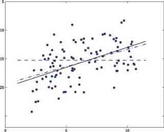
Fig. 1 The simulated data of the example, except for the only outlier which is too far away to be nicely plotted in this figure. Also shown in this figure are the true line of regression (solid line), the line by the LMS solution which has broken down due to the only outlier (dashed line), and the line by the sign-constrained robust estimator to be presented later in Sect. 5 (dash-dotted line). The horizontal and vertical axes show the values of xi and yi , respectively In other words, we have to deal with at least 50% of data contamination in the stress inversion from earthquake focal mechanisms. In image processing, we have also seen a lot of noise other than signal. In this section, we will assume that we have some (rough) prior information about the nature of outŁliers or bad data. By incorporating the prior information into robustness, we will naturally develop the concept of subjecŁtive breakdown point, which might be thought of as a kind of extension or realization of stochastic breakdown proposed by Donoho and Huber (1983). This new breakdown point is said to be subjective, since: (1) it is based on certain prior informaŁtion on the nature of outliers; and (2) such prior information may only reflect the subjective belief of the data analyst on outliers. We will show that a subjective breakdown point can indeed take value beyond the current maximum of 0.5. ConŁsequently, the concept of subjective breakdown point may be meaningfully used to interpret solutions to problems with more than 50% contamination physically. For simplicity of discussion, assume in the linear model
Although the magnitude of the shift dyi can take on any large number, we assume that the sign of Ādyi Āhas a Bernoulli distribution, namely:
- ŃõÕ
(see e.g. Mood et al. 1974), where f(s) is the probability of s positive δyi and (m - s) negative δyj (j ≠ i). It is well known that if m ≥ [n/2] +1, robust procedures will break down, where [x] stands for the integer around but smaller than x. The question of interest now is: with what probability will a robust procedure break down? If a robust method breaks down almost surely or with a large probabilŁity, we can no longer trust and physically interpret the results from the set of contaminated data. On the contrary, if a robust method would break down only with a very small probability, we know that it hardly breaks down and will have confidence in the computed results from contaminated data either for interpretation or practical use. Obviously, the arithmetic mean of the samples will alŁways break down if m ≥ 1, no matter whether we have the prior information (4) or not. It is nowhere robust. In the rest of this section, we will focus on the sample median and the α-trimmed mean. As the first example, let us examine the sample median. It is well known that the median does not break down if m ≤ [n/2](n odd) or m < [n/2](n even). Thus we will focus on [n/2] + 1 ≤ m ≤ n.Given n,m(≥ [n/2] + 1) and p, we know the subjective breakdown point of the median is equal to m/n(> 0.5) and we can compute the probability for this breakdown point as follows:
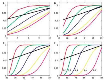
Fig. 2 The subjective breakdown points of the
sample median and their corresponding probabilities of breakdown. The
horizontal and vertical axes show the number of contaminated data and the
probability of breakdown, respectively. The six curves in each subplot are the
subjective breakdown points of the sample median (black line) and their
corresponding probabilities of breakdown with different probabilities for
positive sign of shifts δyi (red line: p = 0.1; green line:
p = 0.2; blue line: p = 0.3; yellow line:
p = 0.4; and purple-red line: p = 0.5). The
four subplots A, B, C and D correspond to the sizes of samples
11, 21, 51 and 101, respectively
Alternatively, we can also compute the probability that the median does not break down as follows:
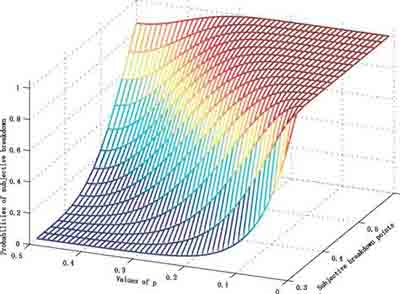
ĀĀ In particular, if p = 1 (ĶļĶ q = 1) and if m≥ [n/2] + 1, then P(breakdown)= 1 or P(not breakdown)= 0. In this special case, we know the median always breaks down with probability one, and it does not make sense to talk about a subjective breakdown point higher than 0.5. In other words, if p = 1 (or q = 1), the median has the maximum breakŁdown point of 0.5. On the other hand, if m ≤ [n/2], then we always have P(breakdown) = 0 or P(not breakdown) = 1, which confirms common sense that the sample median will never break down if the contamination of data is less than 50%. If p = q = 0.5, and let us assume that n = 101 and m = 55, then the subjective breakdown point is 0.5446 and the probability for the median to break down is 2.0474X10⁻¹¹ - an almost zero! If the number of conŁtaminated data is increased to 75, the subjective breakdown point is 0.7426 and the corresponding probability of breakŁdown is still as small as 0.0024442. These two examples have clearly demonstrated that with the prior information (4), the sample median can bear a far more than 50% contaminaŁtion in the data with a negligible probability to break down. In order to see how the subjective breakdown point and its corresponding probability change with p, m and n, we have chosen p = 0.1, 0.2, 0.3, 0.4, 0.5 and n = 11, 21, 51,101, and shown the results in Fig. 2. Obviously, the probability of a subjective breakdown increases rapidly with the decrease of p from 0.5 to 0. However, it decreases significantly with the increase of sample size n. In the ideal situation of p = 0.5, with the increase of samples, the median can bear more perŁcentage of contamination without worrying to break down (compare the purple-red lines in Fig. 2). In the similar manner, we can use (4) to investigate the subjective breakdown point of the α-trimmed mean and its corresponding probability of breakdown. As in the case of the sample median, the subjective breakdown point of the α-trimmed mean can be twice as large as that in the sense of Hampel (1971) and/or Donoho and Huber (1983). For demonstration purpose, we use the third example in Fig. 2 by setting a breakdown point α in the sense of Hampel to 0.3. The subjective breakdown points will then be between 0.3 and 0.6. Since the number of contaminated data is not necessarily an integer, we slightly reduce the size of samples from 51 to 50 such that the product of 50x0.3 makes an integer. The probabilities of subjective breakdown points are shown in Fig. 3.
Fig. 3 Probabilities of
subjective breakdown points of the α-trimmed mean with respect to
subjective breakdown points and p. Here the breakŁdown point α is
0.3 (in the sense of Hampel). The two horizontal axes show the
subjective breakdown points and the probabilities of positive sign of shifts δyi
It can be clearly seen from this figure that if p is between 0.3 and 0.5, then the α-trimmed mean has a good subjective breakdown point of up to 0.5, although the original breakdown point is only 0.3 (in the sense of Hampel). In other words, the α-trimmed mean can bear more contamŁination in the data if the signs of outliers follow the binomial distribution with p sufficiently close to 0.5. The subjective breakdown points of other robust estimators and their corŁresponding probabilities of (subjective) breakdown can be studied in the similar manner but will be omitted here. |


