Least-squares variance component estimation
Authors P.J.G. Teunissen, A.R. Amiri-Simkooei, "Journal of Geodesy", 2008, vol. 82, num. 2, p. 65-82, fragment
Abstract. Least-squares variance component estimation (LS-VCE) is a simple, flexible and attractive method for the estimation of unknown variance and covariance components. LS-VCE is simple because it is based on the well-known principle of LS; it is flexible because it works with a userdefined weight matrix; and it is attractive because it allows one to directly apply the existing body of knowledge of LS theory. In this contribution, we present the LS-VCE method for different scenarios and explore its various properties. The method is described for three classes of weight matrices: a general weight matrix, a weight matrix from the unit weight matrix class; and a weight matrix derived from the class of elliptically contoured distributions. We also compare the LS-VCE method with some of the existing VCE methods. Some of them are shown to be special cases of LS-VCE. We also show how the existing body of knowledge of LS theory can be used to one's advantage for studying various aspects of VCE, such as the precision and estimability of VCE, the use of a-priori variance component information, and the problem of nonlinear VCE. Finally, we show how the mean and the variance of the fixed effect estimator of the linear model are affected by the results of LS-VCE. Various examples are given to illustrate the theory.
2 Weighted least-squares estimation of (co)variance components
2.1 The linear (co)variance component model
First, we will show how one can formulate a linear system of observation equations for the unknown (co)variance components. We start from the linear model
 |
(1) |
with
 |
(2) |
and where E{.} and D{.} denote the mathematical expectation operator and dispersion operator, respectively. The model in Eq. (1) contains two sets of unknowns: the parameter vector x and the (co)variance components ak , k = 1, . . . , p.
It is the goal of VCE to construct an estimator for the unknown (co)variance components. The m¤n matrix A is assumed known and to be of full column rank. Also the cofactor matrices Qk , k = 0, . . . , p, are assumed known and their weighted sum
is assumed to be positive definite. Matrix Q0 is the known part of the variance matrix Qyy.
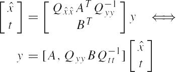
We now introduce a one-to-one transformation of the vector of observables y, such that Eq. (1) takes a simplified form. Let B be a basis matrix of the null space of AT. Thus, B is an m¤(m-n) matrix of which the m n linear independent columns span the null space of AT:ATB = 0 or BTA = 0. Then the following one-to-one correspondence between y and (xT, tT)T exists:
 |
(3) |
with
If we apply this one-to-one transformation to Eq. (1), we obtain the linear model
 |
(4) |
Note the decoupling between x and t. We recognize the n-vector x as the best linear unbiased estimator (BLUE) of x. The zero-mean (m-n)-vector t is the redundancy vector of disclosures. It consists of the misclosures that follow from using the model of condition equations, BTE{y} = 0. The redundancy of the linear model in Eq. (1) is defined as b = m - n. The vector of misclosures t exists on account of redundancy (b > 0). The two random vectors x and t are uncorrelated. They are independent if y is normally distributed.
From Eqs. (2) and (4), it follows, since E{t} = 0 and
that
This equation can be seen as a matrix observation equation for the unknown (co)variance components. The matrix equation consists of b² scalar observation equations. We can bring the matrix observation equation into the familiar vector-matrix form, if we stack the b number of b¤1 column vectors of E {ttT - BTQ0B} into a b²¤1 observation vector. This is achieved by the so-called vec-operator.
However, since the observation matrix ttT - BTQ0B is symmetric, we should only consider the 1/2b(b+1) entries on and below the diagonal of the observation matrix. Otherwise an unwanted duplication of the data occurs. This implies that we should use the vh operator, instead of the vec operator (for a definition and properties of the vec and vh operators, we refer to Appendix A). The use of the vh operator, instead of the vec operator, also avoids the problem of having to work with a singular variance matrix. The variance matrix of vec(ttT) is singular due to the duplication that occurs in the entries of ttT. With the vh operator, we can bring the matrix observation equation in the familiar vector-matrix form of linear observation equations
 |
(5) |
where
The linear model of Eq. (5) will form the basis of our least-squares (co)variance component estimation. The 1/2b(b + 1) vector yvh = vh(ttT - BTQ0B) plays the role of the observation vector. Thus,we have 1/2b(b+1) observation equations in the p unknown parameters ak , k = 1, . . . , p. We will assume that the design matrix of Eq. (5) has full column rank p. The redundancy of the above model is then 1/2b(b + 1) - p.
2.2 The weighted least-squares (co)variance component estimator
Now that we have the above linear model available, we can immediately determine the weighted least-squares solution for the unknown (co)variance components.
Theorem 1 (weighted LS-VCE)
Let
 |
(6) |
be the linear (co)variance component model and define the weighted LS-VCE of
where Wvh is the weight matrix. Then
 |
(7) |
Proof Follows from standard least-squares theory.
The weighted LS-VCE a has many attractive features. Since a is a least-squares estimator, we can make a direct use of the existing body of knowledge of least-squares theory. This holds true for the numerical aspects (e.g., use can be made of standard least-squares software packages), as well as for many of the statistical aspects.
First we give, for later use, two different but equivalent expressions for the LS-VCE system of normal equations.
Corollary 1 (LS-VCE normal equations)
Let the system of normal equations of the LS-VCE of Eq. (7) be given as
 |
(8) |
with normal matrix
and right-hand side
Then the entries nkl of the normal matrix N and the entries rk of the right-hand side vector r, are given as
 |
(9) |
and
 |
(10) |
with D the duplication matrix, D+ its pseudo-inverse, ci the canonical unit vector having a one as its i th entry, and
(for a definition of the Kronecker product and duplication matrix and their relations with the vec and vh operator, we refer to Appendix A).
Proof From
and vh(.) = D+vec(.) the first part is trivial. One can now rewrite the b² ¤ b² matrix D+TWvhDT as the sum
with
the appropriate b ? b submatrices. Substitution of this expression gives
In a similar way, the right-hand side rk is obtained.


