Alina Stikhar
Faculty: Computer Information Technologies and Automation
Department: Automated Control Systems
Speciality: Information Control System and Technologies
Theme of Master's Work:
Algorithms and methods of computing system
of forecasting population rates
Scientific Supervisor: Ph. D. Maxim V. Privalov

of forecasting population rates»
RELEVANCE
This topic is always actual since demographic forecasts are used as a basis for planning more often. For example, at an estimation of requirements of the country or region in new workplaces, teachers, schools, doctors, medical sisters, city habitation or a foodstuff, it is necessary to have data on a population to which services will be necessary. Thus, demographic forecasts serve as a starting point for the majority of forecasts about the future requirements.

PURPOSE AND TASKS OF DESIGH AND RESEARCH
The purpose is to justify and select a method of forecasting of a population indexes in the conditions of a possible modification of factors, and to develop algorithms of computerization system of forecasting of a population indexes.
Research problems are:
• To carry out mathematical formalising of the task of forecasting with varying conditions of sets of factors;
• To carry out statement of the problem of an experimental research of an exactitude of methods;
• To fulfil program implementation;
• To research experimentally the accuracy of operation of methods of decision trees and neural networks, under condition of a modification of sets of factors;
• To develop algorithm and the software on the basis of the selected method.
Subject of development and research is forecasting methods.
The object of development and research is the task of forecasting of demographic indexes.
Methods of research are the neural networks and decision trees.

MATHEMATICAL STATEMENT OF PROBLEM
Neural networks are a section of an artificial intelligence in which for handling phenomena’s signals are used, similar to those events in neurons of live beings.
The approximation of functions is one of the most general use of artificial neural networks. The general framework of the approximation problem is the following. One supposes the existence of a relation between several input variables and one output variable. Without knowing this relation, one tries to build an approximator (black box model) between these inputs and this output. The structure of this approximator must be chosen and the approximator must be calibrated to best represent the input-output dependence. To realize these different stages, one disposes of a set of inputs-output pairs that constitute the learning data of the approximator.
In master's work, for solution of the forecasting task, as the neural network architecture the radial basis network (RBF) has been selected on which input the many-dimensional time series will be moved given. The result of forecasting is value of time series in a demanded time measurement.
It is necessary to make a prognosis for improvement of quality of preliminary information processing. As neural networks badly work with values from a wide range of the values meeting in input data. For elimination of this undesirable appearance data it is necessary to scale in a range [0... +1] or [-1... +1]. The formula looks like the following:
 |
(1) |
 |
(2) |
 |
(3) |
Where  – accordingly, the scaled and initial input data;
 – a maxima and a goal function minimum;
 – a maxima and a minimum of input data.
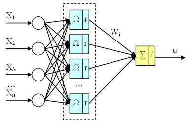
The radial basis neural network (fig. 1) a network with one hidden layer:

Figure 1 – Representation of a RBFN
We dispose of a set of inputs xt and a set of outputs yt. The approximation of y, by a RBFN will be noted ўt. This approximation will be the weighted sum of m Gaussian kernels Φ:
 |
(4) |
| t = 1 to N , with | |
 |
(5) |
The complexity of a RBFN is determined by the number of Gaussian kernels. The different parameters to specify are the position of the Gaussian kernels (Ci), their variances (σi), and the multiplicative factors (λi).
The position of the Gaussian kernels is chosen according to the distribution of xt in space. At locations where there are few inputs xt few nodes will be placed and conversely, a lot of nodes will be placed where there are many input data.
The technique that allows realizing this operation is called vector quantization and the points that summarize the position of the nodes are called centroids. The vector quantization is composed of two stages. The centroids are first randomly initialized in the space. They are then placed in the following way. All xt points are inspected, and for each of them the closest centroid will be moved in the direction of xt according to the following formula:
 |
(6) |
with xt the considered point, Ct the closest centroid to xt, and α a parameter that decreases with time.
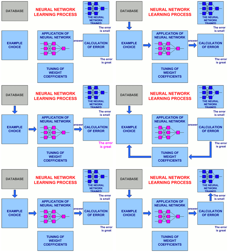
In a fig. 2 the generalised circuit of procedure of training of a neural network is presented.

Figure 2 – The General view of procedure of training of a neural network
(animation: volume – 32 864 byte; size – 450х295; consists of 16 frames;
a delay between last and the first frames – 1 000 msec;
a delay between frames – 700 msec; quantity of recycle – continuous)
The model presented in the form of decision tree, is intuitively clear and simplifies understanding of the being solved task. The algorithm of designing of a decision tree does not demand from the user to choose of entry attributes (independent variable). It is possible to give all existing attributes on an algorithm input. The algorithm itself will select the most significant one among them, and only they will be used for tree construction. For example, In comparison with neural networks, it considerably facilitates operation because in neural networks the choice of an amount of entry attributes essentially reduces training time.
The majority of algorithms of decision trees’ designing have possibility of special handling of the skipped values.
In the work the scaled algorithm of decision trees is SLIQ is used, i.e. the target variable has continuous values. Thus, SLIQ allows to instal dependence of a target variable on independent (entry) variables.
For tree construction the following algorithm is used. There is a data table X, in which n attributes (to each column of attribute  , it is attached the column with indexes
  ), and Y – a target variable. Firstly it is necessary to fulfil sorting of each numerical attribute, and independently from each other in this connection, it is necessary to store indexes.

Let's accept  – the sorted values of numerical attribute
  . As, any value between
  and
and  will divide set into the same two subsets, it is necessary to research only n-1 a possible partition. The middle of each interval
  and
and  is considered a possible point of a partition (i.e. a possible nodes).
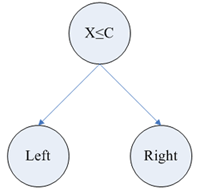
In algorithm SLIQ each nodes of a decision tree has two “offsprings”. On each step of construction of a tree the sort rule  , formed in a nodes, divides set learning sampling into two parts – a part in which the rule is fulfilled right “offspring” and the part in which the rule is not fulfilled left “offspring”. Fig. 3 illustrates all the aforesaid.

Figure 3 – The Example of decision tree
For a choice of an optimal rule the function of an estimation of a partition quality is used which is defined as minimisation SSE (7):
 |
(7) |
 |
(8) |

LIST OF USED LITERATURE
1. John Stover DemProj Version 4 A Computer Program for Making Population Projections: March 2007. – 106 с.
2. Учебник. Методы прогнозирования: Регрессионные методы прогнозирования [Электронный ресурс] / Аналитические технологии для прогнозирования и анализа данных. НейроПроект: 1999-2005. Режим доступа: URL:
http://www.neuroproject.ru/forecasting_tutorial.php
3. Комарцова Л.Г. Нейрокомпьютеры: Учеб. пособие для вузов. – 2-е изд., перераб. и доп. – М.: Изд-во МГТУ им. Н.Э. Баумана, 2004. – 400с.
4. Прогнозирование и классификация экономических систем в условиях неопределенности методами искусственных нейронных сетей: Аналитический обзор. [Электронный ресурс]. Режим доступа:
URL: http://www.nauka-shop.com/mod/shop/categoryID/110/page/34
5. Чубукова И.А. Методы классификации и прогнозирования. Деревья решений: конспект лекций. [Электронный ресурс]: Режим доступа: URL: http://www.intuit.ru/department/database/datamining/9/2.html
6. Временной ряд. Глоссарий. [Электронный ресурс] / Режим доступа: URL: http://www.basegroup.ru/glossary/definitions/time_series/
7. Wasserman P.D. Neural Computing: Theory and Practice / Van Nostrand Reinhold, New York, NY 1989. – 189 с.
8. Lendasse А. Approximation by radial basis function networks application.
9. А. Шахиди Деревья решений – общие принципы работы. [Электронный ресурс]. Режим доступа: URL: http://www.basegroup.ru/library/analysis/tree/description/
10. Manish Mehta, Rakesh Agrawal, Jorma Rissanen SLIQ: A Fast Scalable Classifier for Data Mining. / IBM Almaden Research Center, – 15 с.
While writing the given abstract the master's work has not been completed yet. The final date of the work completed is December, 1st, 2009. The text of master's work and materials on this topic can be received from the author or her research guide after the indicated date.


