
Автор: Bill Green
Название статьи: Canny Edge Detection Tutorial
Источник: Drexel Autonomous Systems Lab., 2002.
http://www.pages.drexel.edu/~weg22/can_tut.html
This tutorial will teach you how to:
(1) Implement the Canny edge detection algorithm.


Edges characterize boundaries and are therefore a problem of fundamental importance in image processing. Edges in images are areas with strong intensity contrasts – a jump in intensity from one pixel to the next. Edge detecting an image significantly reduces the amount of data and filters out useless information, while preserving the important structural properties in an image. This was also stated in my Sobel and Laplace edge detection tutorial, but I just wanted reemphasize the point of why you would want to detect edges.
The Canny edge detection algorithm is known to many as the optimal edge detector. Canny's intentions were to enhance the many edge detectors already out at the time he started his work. He was very successful in achieving his goal and his ideas and methods can be found in his paper, "A Computational Approach to Edge Detection". In his paper, he followed a list of criteria to improve current methods of edge detection. The first and most obvious is low error rate. It is important that edges occuring in images should not be missed and that there be NO responses to non-edges. The second criterion is that the edge points be well localized. In other words, the distance between the edge pixels as found by the detector and the actual edge is to be at a minimum. A third criterion is to have only one response to a single edge. This was implemented because the first 2 were not substantial enough to completely eliminate the possibility of multiple responses to an edge.
Based on these criteria, the canny edge detector first smoothes the image to eliminate and noise. It then finds the image gradient to highlight regions with high spatial derivatives. The algorithm then tracks along these regions and suppresses any pixel that is not at the maximum (nonmaximum suppression). The gradient array is now further reduced by hysteresis. Hysteresis is used to track along the remaining pixels that have not been suppressed. Hysteresis uses two thresholds and if the magnitude is below the first threshold, it is set to zero (made a nonedge). If the magnitude is above the high threshold, it is made an edge. And if the magnitude is between the 2 thresholds, then it is set to zero unless there is a path from this pixel to a pixel with a gradient above T2.
Step 1
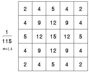
In order to implement the canny edge detector algorithm, a series of steps must be followed. The first step is to filter out any noise in the original image before trying to locate and detect any edges. And because the Gaussian filter can be computed using a simple mask, it is used exclusively in the Canny algorithm. Once a suitable mask has been calculated, the Gaussian smoothing can be performed using standard convolution methods. A convolution mask is usually much smaller than the actual image. As a result, the mask is slid over the image, manipulating a square of pixels at a time. The larger the width of the Gaussian mask, the lower is the detector's sensitivity to noise. The localization error in the detected edges also increases slightly as the Gaussian width is increased. The Gaussian mask used in my implementation is shown below.
Step 2
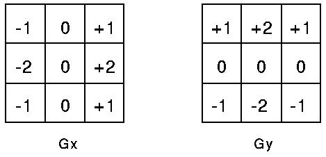
After smoothing the image and eliminating the noise, the next step is to find the edge strength by taking the gradient of the image. The Sobel operator performs a 2-D spatial gradient measurement on an image. Then, the approximate absolute gradient magnitude (edge strength) at each point can be found. The Sobel operator uses a pair of 3x3 convolution masks, one estimating the gradient in the x-direction (columns) and the other estimating the gradient in the y-direction (rows). They are shown below:
The magnitude, or EDGE STRENGTH, of the gradient is then approximated using the formula:
Step 3
Finding the edge direction is trivial once the gradient in the x and y directions are known. However, you will generate an error whenever sumX is equal to zero. So in the code there has to be a restriction set whenever this takes place. Whenever the gradient in the x direction is equal to zero, the edge direction has to be equal to 90 degrees or 0 degrees, depending on what the value of the gradient in the y-direction is equal to. If GY has a value of zero, the edge direction will equal 0 degrees. Otherwise the edge direction will equal 90 degrees. The formula for finding the edge direction is just:
Step 4
Once the edge direction is known, the next step is to relate the edge direction to a direction that can be traced in an image. So if the pixels of a 5x5 image are aligned as follows:
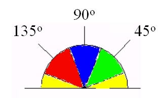
Therefore, any edge direction falling within the yellow range(0 to 22.5 & 157.5 to 180 degrees) is set to 0 degrees. Any edge direction falling in the green range (22.5 to 67.5 degrees) is set to 45 degrees. Any edge direction falling in the blue range (67.5 to 112.5 degrees) is set to 90 degrees. And finally, any edge direction falling within the red range (112.5 to 157.5 degrees) is set to 135 degrees.
Step 5
After the edge directions are known, nonmaximum suppression now has to be applied. Nonmaximum suppression is used to trace along the edge in the edge direction and suppress any pixel value (sets it equal to 0) that is not considered to be an edge. This will give a thin line in the output image.
Step 6
Finally, hysteresis is used as a means of eliminating streaking. Streaking is the breaking up of an edge contour caused by the operator output fluctuating above and below the threshold. If a single threshold, T1 is applied to an image, and an edge has an average strength equal to T1, then due to noise, there will be instances where the edge dips below the threshold. Equally it will also extend above the threshold making an edge look like a dashed line. To avoid this, hysteresis uses 2 thresholds, a high and a low. Any pixel in the image that has a value greater than T1 is presumed to be an edge pixel, and is marked as such immediately. Then, any pixels that are connected to this edge pixel and that have a value greater than T2 are also selected as edge pixels. If you think of following an edge, you need a gradient of T2 to start but you don't stop till you hit a gradient below T1