E&F CHAOS: A USER FRIENDLY SOFTWARE PACKAGE FOR NONLINEAR ECONOMIC DYNAMICS

Cees Diks, Cars Hommes, Valentyn Panchenko, Roy van der Weide

Quantitative Finance, Center for Nonlinear Dynamics in Economics and Finance (CeNDEF)

A Higher Dimensional Example

  In this section we consider a higher dimensional example of a nonlinear system, to illustrate more features of the E&F Chaos software. The model is an extension of the agent-based cobweb model with heterogeneous expectations (rational versus naive expectations) introduced by Brock and Hommes (1997), modified to allow for asynchronous updating of strategies. This extension allows us to illustrate how easy it is to include a new or extended model in E&F Chaos. As in the previous section, demand is linear and given by

D(pt ) = a - bpt .

  The supply is also assumed to be linear, derived from expected profit maximization from a quadratic cost function c(q) = q²/(2s), and therefore given by

S(p(ht)^e) = s*p(ht)^e ,

  where p(ht)^e is the expected market price by agents of type h. Agents can choose between two different types of expectation rules, a costly sophisticated rule and a cheap free rule. The type 1 rule is rational expectations, which can be obtained at information gathering costs C > 0, while the type 2 rule is naive expectations, which is available at no cost. The forecasting rules thus are

p(1t)^e = p(t),    p(2t)^e= pt-1.

  With rational and naive producers, the market clearing condition is given by

a - b*p(t) = n(1t)*s*p(t) + n(2t)*s*p(t-1),

  where n(1t) and n(2t) represent the fractions of type 1 and type 2 agents. The unique market clearing price pt is then given by

p(t) = (a - n(2t)*s*p(t-1))/(b + s*n(1t)).

  The fractions are determined by the past performance of the two forecasting strategies. The payoff Ï(ht) of strategy h at time t is given by the realized profit of that strategy at time t minus the costs incurred. Using producers’ quadratic cost function c(q) = q²/(2s) and taking the constant information gathering costs C > 0 for rational expectations into account, one finds

Ï(1t) = b2*p2(t) - C, Ï(2t) = b2*p(t-1)*(2p(t) - p(t-1)).

  The fitness measure U(ht) of strategy h is a geometrically downweighted average of past profits, i.e.

U(ht) = w*U(h,t-1) + (1 - w)*Ï(ht) ,

  where w ª [0, 1) is a memory parameter. The extreme case w = 0 represents agents basing their evaluation only on the profits observed in the previous period. Brock and Hommes (1997) considered this model with synchronous updating of strategies, that is, in each period all agents update their strategies. Here we consider themore general case of asynchronous updating. Per time unit only a fraction 1 - δ of agents, distributed randomly among agents of both types and independently across time, is assumed to reconsider their strategy on the basis of the most recent information available. The remaining fraction δ continues to use their previous strategy. The corresponding dynamics of the fractions is given by a modified version of the discrete choice, logit probabilities:

n(ht) = (1 - δ)*e*β*U(h,t-1)/Z(t-1) + δn(h,t-1),

  where Z(t-1) = ÑÓÌÌ h^e*β*U(h,t-1) is a normalization factor so that the fractions add up to 1. For δ = 0, we are back in the case of synchronous updating. In evolutionary game theory there has been a discussion whether asynchronous updating may lead to more stability (cf. Nowak and May 1992; Huberman and Glance 1993; Nowak et al. 1992). Financial market models with asynchronous updating have been considered by Diks and van der Weide (2005) and Hommes et al. (2005).

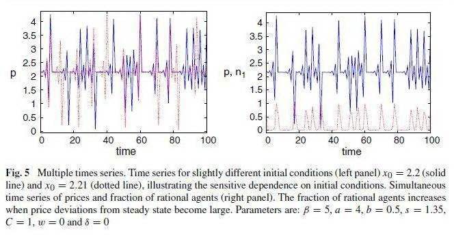
  The dynamics of the cobweb model with rational versus naive agents and asynchronous updating of strategies is thus given by Eqs. 10–13, defining a nonlinear four-dimensional (with state variables p(t-1), n(1,t-1), U(1,t-1) and U(2,t-1) discrete time dynamical system. A typical research question for such a generalization of an existing model is how the extra parameters affect the dynamics. Our aim is to illustrate how the E&F Chaos program can help to obtain a quick overview of the (long-run) behavior of the dynamics in different regions of the parameter space.

Building a New Model in E&F Chaos

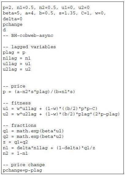
  Including a new model or modifying an existing model in the E&F Chaos software is easy. All the user has to do is to specify the model in LUA code (or modify an existing model) in a plain text file, either with the built-in editor or with her own favorite editor. To view an example, the user can use the File/Load Model submenu, open the subdirectory "My Models" and select the file "BH-cobweb-async", the cobweb model with asynchronous updating as presented in the previous subsection. Using the File/Edit Model submenu, a window containing the model equations appears: