Theme of master's work:
ĢSimulation of complex mechanical systems in package DYMOLA / MODELICAģ
1 Introduction
2 Simulating a model industrial robot
3 REFERENCES
This chapter will take you through some examples in order to get you started with Dymola.
For detailed information about the program, you are referred to the on-line documentation
and the users manuals. The on-line documentation is available in the Help menu after selecting
Documentation. The tool tips and the Whats this feature are fast and convenient
ways to access information.
Start ĢDymolaģ,. A Dymola window appears. A Dymola window operates in one of the two
modes:
Modeling for finding, browsing and composing models and model components.
Simulation for making experiments on the model, plotting results, and animating behavior.
Dymola starts in Modeling mode. The active mode is selected by clicking on the tabs in the
bottom right corner of the Dymola window.
The operations, tool buttons available, and types of sub-windows appearing depends on the
mode, and additional ones have been added after this guide was written. Dymola starts with
a useful default configuration, but allows customizing.
This first example will show how to browse an existing model, simulate it, and look at the
results. If you want to learn the basics first, you can skip to a smaller example in the next
section Solving a non-linear differential equation.
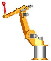
We will study a model of an industrial robot. Start Dymola. The Dymola window appears in
Modeling mode as displayed above. To view the industrial robot model, use the File/Demos
menu and select Robot.
Dymola starts loading the Ģmodel librariesģ needed for the robot model and displays it.
The package browser in the upper left sub-window displays the package hierarchy and it is
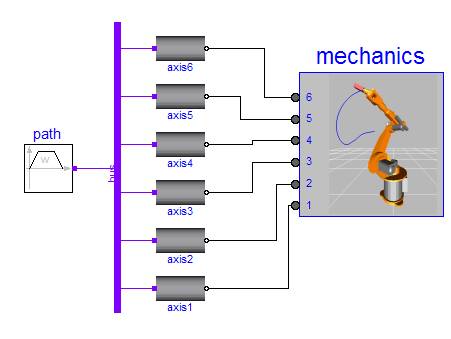
now opened up with the robot model selected and highlighted. The model diagram in the
right sub-window opens up and shows the top-level structure of the model. The model diagram
has an icon for the model of the robot with connected drive lines for the joints. The
reference angles to the drive lines are calculated by a path planing module giving the fastest
kinematic movement under given constraints.
The component browser in the lower left sub-window also shows the components of the robot
experiment in a tree structured view.
To inspect the robot model, select the icon in the Diagram window (red handles appear, see
below) and press the right button on the mouse.
It is not necessary to select the robot component explicitly by pressing the left button on the
mouse to access its menu. It is sufficient to just have the cursor on its icon in the diagram
window and press the right button on the mouse. The component browser also gives easy
access to the robot component. Just position the cursor over mechanics. The component
browser provides a tree representation of the component structure. The diagram window
and the component browser are synchronized to give a consistent view. When you select a
component in the diagram window, it is also highlighted in the component browser and vice
versa. The diagram window gives the component structure of one component, while the
component browser gives a more global view; useful to avoid getting lost in the hierarchical
component structure.
The Diagram window now displays the mechanical structure consisting of connected joints
and masses. The component browser is opened up to also show the internals of the mechanics
model component.
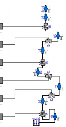
Double click on, for example, r1 at the bottom of the diagram window. This is a revolute
joint. The Parameter dialogue appears. The Parameter dialogue can also be accessed from
the right button menu. Double clicking the left button selects the first alternative from the
right button menu.
To learn more about this component, select Info. An HTML browser is opened to show the
documentation of the Revolute joint.
If you do only want to see the documentation select the component in the diagram, press the
right mouse button and select Info. An HTML browser is opened to show the documentation
of the Revolute joint. By double clicking on the other components, you can, for example,
see what parameters a mass has.
Let us now inspect the drive train model. There are several possible ways to get it displayed.
Press the Previous button (the toolbar button with the bold left arrow) once to go to
the robot model and then use the right button menu on one of the axis icons. Please, note
that robot.mechanics also has components axis1, ..., axis6, but those are just connectors.
You shall inspect for example robot.axis1. Another convenient way is to use the component
browser and use the right button menu and select Show Component. Since this is the first
menu option, double clicking will open up the component in the Diagram window. Please,
recall that double clicking on a component in the diagram window pops up the parameter
dialogue.
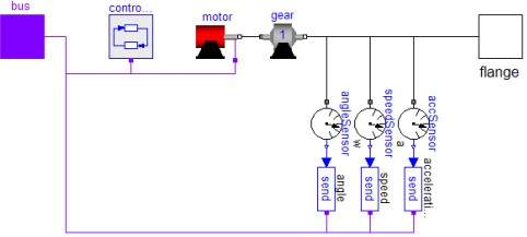
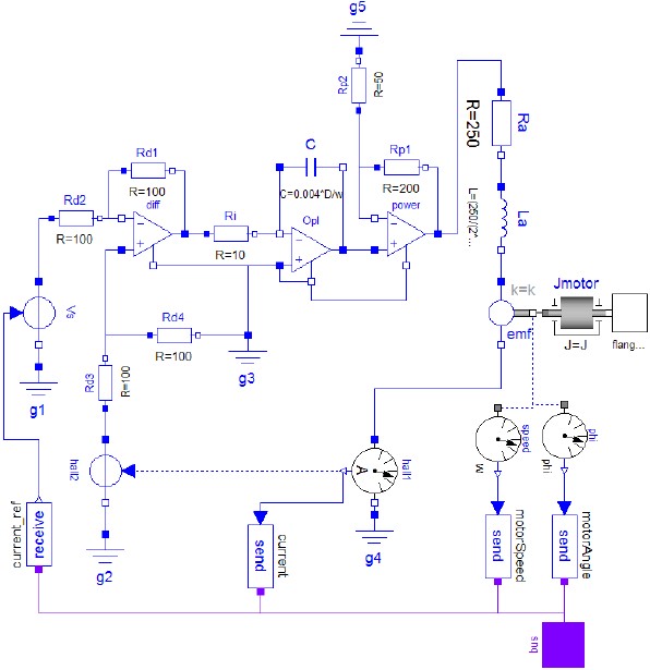
The drive train includes a controller. A data bus is used to send measurements and reference
signals to the controller and control signals from the controller to the actuator.
The bus for
one axis has the following signals: - angle_ref(reference angle of axis flange),
- angle(angle of axis flange),
- speed_ref(reference speed of axis flange),
- speed(speed of axis flange),
- acceleration_ref(reference acceleration of axis flange),
- acceleration(acceleration of axis flange),
- current_ref( reference current of motor),
- current( current of motor),
- motorAngle( angle of motor flange),
- motorSpeed(speed of motor flange
).
There are send elements to output information to the bus as illustrated in the model diagram
above. Similarly there are a read elements to access information from the bus.The bus from the path planning module is built as an array having 6 elements of the bus for
an axis.
The bus from the path planning module is built as an array having 6 elements of the bus for
an axis.
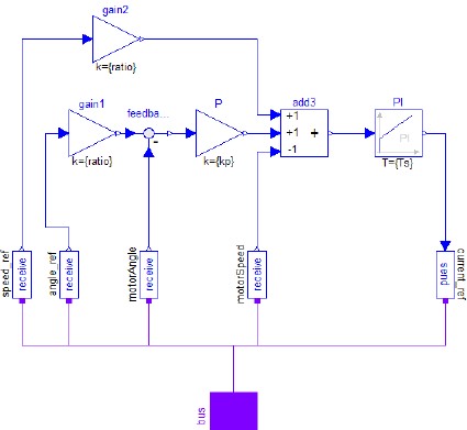
The controller of an axis gets references for the angular position and speed from the path
planning module as well as measurements of the actual values of them. The controller outputs
a reference for the current of the motor, which drives the gearbox.
The motor model consists of the electromotorical force, three operational amplifiers, resistors,
inductors, and sensors for the feedback loop.
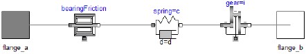
View the component gear in a similar way as for the other components. It shows the gearbox
and the model of friction of the bearings and elasticity of the shafts.
Let us simulate the robot model. To enter the Simulation mode, click on the tab at the bottom
right. When you selected the robot the Commands menu became active to indicate that
robot contains a Command for simulating it, select this.In addition the simulation menu includes commands to setup and run simulations. The Setup
menu item opens a dialogue allowing the setting of start and stop times. The icon indicates
which toolbar button to use for quick access to the set up dialogue. The Simulate
menu item starts a simulation.
In this case, however, a command script has been prepared. To run the script, select Commands
select Simulate. Dymola then translates the model and simulates automatically.
The animation window is opened automatically, because the simulation result contains animation
information.
It is possible to change the viewing position by opening a view controller, Animation/3D
View Control.
llijknllpkl;
- http://www.Modelica.org
Modelica.
Äîėāøí˙˙ ņōđāíčöā Modelica.
- http://www.Modelica.org/tools.shtml
- http://www.actsolutions.it
Číņōđķėåíōû Modelica.
- Dierk Schroder. ElektrischeAntriebe Regelung von Antriebssystemen. Technische Universitat Munchen
- . J. McPhee, C. Schmitke, S. Redmond. Dynamic modelling of mechatronicmultibody systems with symbolic computing and linear graph theory. Mathematical and Computer Modelling of Dynamical Systems, 10(1): 1 23, 2004.
- Michael Tiller wrote the first book on Modelica with the title "Introduction to Physical Modeling with Modelica" (May 2001).
- Peter Fritzson - "Principles of Object-Oriented Modeling and Simulation with Modelica 2.1" (November 2003)
|
