Continuous LOD Terrain Meshing
Using Adaptive Quadtrees
by Thatcher Ulrich
Revised February 28, 2000
Source of information: http://www.gamasutra.com/view/feature/3434/continuous_lod_terrain_meshing_.php
Terrain rendering is a perennial hot issue in the world of game programming. Right now we're at a particularly interesting point in the development of terrain rendering technology, because polygon budgets have risen to the point where, in conjunction with real-time LOD meshing algorithms taken from published academic papers, state-of-the-art game engines are able to draw quite a bit of reasonably detailed terrain. However, the techniques which are currently in common use must compromise either on terrain size or on close-up detail.
As part of the R&D for Soul Ride, the game I'm currently working on (http://www.soulride.com ), I experimented with the published algorithms, and eventually came up with an extension that eliminates the tradeoff between terrain size and close-up detail. This article presents my algorithm, along with its similarities and differences from the above-mentioned algorithms.
I'll start by reviewing the problem of terrain rendering, and describe the problem solved by [1], [2], and [3] (see references at the end of this article). Then I'll explain the additional problem solved by my algorithm. I'll present a detailed description of the algorithm, and discuss some of the problems with it and some of the untapped potential. And last but not least, I'll provide the source code to a demo that implements my algorithm, which you can use to help understand it, evaluate its effectiveness, and incorporate directly into your own projects if you want.
This article is not a general tutorial or review of terrain rendering. I'm going to assume some familiarity on your part with the problem. If things aren't making much sense, you may want to consult the excellent references listed at the end of the article.
The Problems
What do we want from a terrain renderer? We want a single continuous mesh from the foreground all the way to the horizon, with no cracks or T-junctions. We want to view a large area over a large range of detail levels: we want to see the bumps in front of our feet to the mountains in the background. For the sake of discussion, let's say that we want feature size to range from 1m up to 100000m; five orders of magnitude.
How can we do it? The brute-force approach won't work on ordinary computers circa Y2K. If we make a 100000m x 100000m grid of 16-bit height values, and just draw them in a mesh (Figure 1), we'll end up with two big problems.First, the triangle problem: we'll be sending up to 20 billion triangles/frame to our rendering API. Second, the memory problem: our heightfield will consume 20 GB of data. It will be many years before hardware advances to the point where we can just use brute-force and get good results.
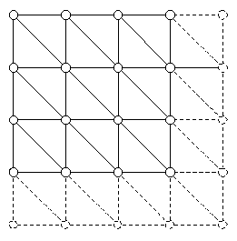
Fig.1 - Brute force approach to a heightfield mesh.
There are several previously-published methods which successfully tackle the triangle problem. The most widely used ones employ a clever family of recursive meshing algorithms [1], [2], [3]. Using one of these algorithms, we can effectively tame our mesh, and render a seamless terrain with a few thousand triangles, with the vertices intelligently selected on the fly from the 10 billion in the dataset.
However, we still have a memory problem, since the heightfield dataset consumes 20 GB (plus some overhead to support the meshing algorithm).
One obvious solution is to compromise on detail by making the heightfield dimensions smaller. 1k x 1k is a good practical size for a heightfield with today's machines. A recently released game called TreadMarks uses a 1k x 1k dataset to excellent effect [4] (see references at the end of the article). Unfortunately, 1k x 1k is still a far cry from 100k x 100k. We end up having to limit either the size of the terrain and the view distance, or the amount of foreground detail.
The solution which I cover in this article is to use an adaptive quadtree, instead of a regular grid, to represent the terrain height information. Using this quadtree, we can encode height data at different resolutions in different regions in the terrain. For example, in a driving game, you would want lots of fine detail on and around the roads, ideally showing every bump, but you wouldn't need that much detail for the surrounding wilderness that you can't drive to; you only need enough detail for the general shape of hills and valleys.
The quadtree can also be used for another attack on the memory problem: procedural detail. The idea is to pre-define the shape of the terrain at a coarse level, and have the computer automatically generate fine detail on the fly for the area immediately around the viewer. Because of the quadtree's adaptive nature, this detail can be discarded when the viewer moves, freeing up memory for creating procedural detail in a different region.
Separately, the use of quadtrees for adaptive representation of 2D functions, and the use of quadtrees for recursive meshing [1], [3] are both well-known. However, [1] and [3] both use regular grids for their underlying heightfield representation. Extending their meshing approach to work with a true adaptive quadtree presents numerous complications, and requires some tricky programming. Hence this article and the accompanying demo code.
Meshing
My meshing algorithm is based on [1], which has also influenced [2] and [3]. There are a few key modifications, but much of the basic approach is the same, and I borrow a lot of the [1] terminology.
There are two parts to meshing. I call the first part Update() and the second part Render(), after [1]. During Update(), we'll decide which vertices to include in the output mesh. Then, during Render() we'll generate a triangle mesh that includes those vertices. I'll start by explaining Update() and Render() for an extremely simple heightfield: a 3x3 grid (Figure 2). To Update() it, we'll look at each of the optional vertices and decide whether to include them in the mesh. Following the terminology of [1], we'll say that if and only if a vertex is "enabled", then we'll use it in the mesh.
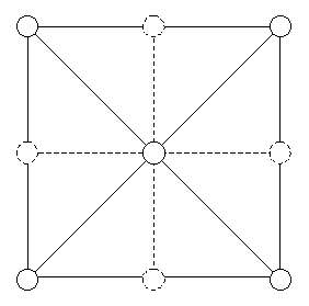
Figure 2. A 3x3 heightfield. Dashed lines and vertices are optional in an LOD mesh.
Take as given that the center and corner vertices are enabled. So the task is to calculate the enabled state for each of the four edge vertices, according to some LOD calculation which takes the viewpoint and the vertex attributes into account.
Once we know which vertices are enabled, we can Render() the mesh. It's easy; we just make a triangle fan with the center vertex as the hub, and include each enabled vertex in clockwise order around the outside. See Figure 3 for examples.
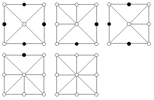
Figure 3. Examples of LOD meshes on the 3x3 heightfield. Disabled vertices in black.
To Update() and Render() an adaptive quadtree heightfield, we extend the above process by starting with that same 3x3 square and recursively subdividing it. By subdividing, we can introduce new vertices, and treat them like we treated the vertices of the original square. In order to prevent cracks, however, we'll have to observe some rules.
First, we can subdivide any combination of the four quadrants. When we subdivide a quadrant, we'll treat the quadrant as a sub-square, and enable its center vertex. For mesh consistency, we will also have to enable the edge vertices of the parent square which are corners of the quadrant (Figure 4). We'll define enabling a square to imply the enabling of its center vertex as well as those corners.
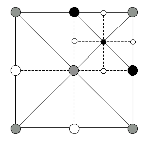
Figure 4. Subdividing the NE quadrant of a square. The gray vertices are already known to be enabled, but the black vertices must be enabled when we subdivide.
Next, notice that an edge vertex in a sub-square is shared with a neighboring sub-square (except at the outside edges of our terrain). So when we enable an edge vertex, we will have to make sure that the neighboring sub-square which shares that vertex is also enabled (Figure 5). Enabling this neighbor square can in turn cause other vertices to be enabled, potentially propagating enabled flags through the quadtree. This propagation is necessary to ensure mesh consistency. See [1] for a good description of these dependency rules.
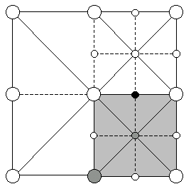
Figure 5. While updating the NE quadrant, we decide to enable the black vertex. Since that vertex is also shared by the SE quadrant (marked in gray), we must enable that quadrant also. Enabling the SE quadrant will in turn force us to enable the gray vertices.
After we're done with the Update(), we can Render() the quadtree. Rendering is actually pretty simple; the complicated consistency stuff was taken care of in Update(). The basic strategy is to recursively Render() any enabled sub-squares, and then render any parts of the square which weren't covered by enabled sub-squares. (Figure 6) shows an example mesh.
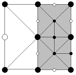
Figure 6. An example mesh. Enabled vertices are marked in black. The gray triangles are drawn by recursive calls to Render() on the associated sub-squares. The white triangle are drawn by the original call to Render().
Evaluating vertices and squares
In the above description, I glossed over the part about deciding whether a vertex should be enabled. There are a few different ways to do this. All of them take into account what I'll call the "vertex interpolation error", or vertex error for short. What this is, is the difference in height between the correct location of a vertex, and the height of the edge in the triangle which approximates the vertex when the vertex is disabled (Figure 7). Vertices which have a large error should be enabled in preference to vertices which have a small error. The other key variable that goes into the vertex enable test is the distance of the vertex from the viewpoint. Intuitively, given two vertices with the same error, we should enable the closer one before we enable the more distant one.
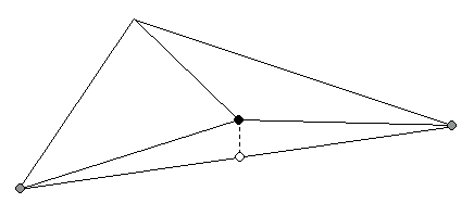
Figure 7. Vertex interpolation error. When a vertex is enabled or disabled, the mesh changes shape. The maximum change occurs at the enabled vertex's position, shown by the dashed line. The magnitude of the change is the difference between the true height of the vertex (black) and the height of the original edge below the vertex (white). The white point is just the average of the two gray points.
There are other factors that can be included as well. [1] for instance takes into account the direction from the viewpoint to the vertex. The justification is based on the idea of screen-space geometric error; intuitively the vertex errors are less visible when the view direction is more vertical. [1] goes through the math in detail.
However, I don't think screen-space geometric error is a particularly good metric, for two reasons. One, it ignores texture perspective and depth buffering errors -- even if a vertex does not move in screen space because the motion is directly towards or away from the viewpoint, the vertex's view-space z value does affect perspective-correction as well as depth-buffering. Two, the viewpoint-straight-down case is both an easy case for terrain LOD algorithms, and not a typical case.
In my opinion, there's no point in optimizing for an atypical easy case in an interactive system. The performance of the more typical and difficult case, when the view axis is more horizontal and much more terrain is visible, will determine the minimum system frame-rate and hence the effectiveness of the algorithm.
Instead of screen-space geometric error, I advocate doing a similar test which results in 3D view-space error proportional to view distance. It's really very similar to the screen-space-error test, but without the issues I mention above. It involves only three quantities: an approximation of the viewpoint-vertex distance called the L1-norm, the vertex error, and a detail threshold constant. Here it is:
L1 = max(abs(vertx - viewx), abs(verty - viewy), abs(vertz - viewz));
enabled = error * Threshold < L1;
You probably recognize the L1-norm, even if you didn't know it had a fancy name. In practice, using the L1-norm instead of the true viewpoint distance will result in slightly more subdivision along the diagonals of the horizontal terrain plane. I've never been able to detect this effect by eye, so I don't worry much about it. [4] and others use view-space-z rather than the L1-norm, which is theoretically even more appropriate than true viewpoint distance. Nevertheless, the L1-norm works like a champ for me, and [3] uses it too.
You can treat the Threshold quantity as an adjust-for-best-results slider, but it does have an intuitive geometric interpretation. Roughly, it means: for a given view distance z, the worst vertex error I'll tolerate is z / Threshold. You could do some view-angle computations and relate Threshold to maximum pixel error, but I've personally never gone past the adjust-for-best-results stage.
So that covers the vertex enabled test. But if you were paying attention earlier, you may also have noticed that I glossed over another point, perhaps more important: during Update(), how do we know whether to subdivide a quadrant or not? The answer is to do what I call a "box test". The box test asks the question: given an axis-aligned 3D box enclosing a portion of terrain (i.e. a quadtree square), and the maximum vertex error contained within that box, and no other information about what's inside the box, is it possible that the vertex enable test would return true? If so, then we should subdivide the box. If not, then there's no reason to subdivide.
The beauty of it is, by doing the box test, we can potentially trim out thousands of vertices from consideration in one fell swoop. It makes Update() completely scalable: its cost is not related to the size of the full dataset, only to the size of the actual data that's included in the current LOD mesh. And as a side benefit, the precomputed vertical box extent can be used during Render() for frustum culling.
The box test is conservative, in that a square's max-error could be for a vertex on the opposite side of the box from the viewpoint, and thus the vertex test itself would/will fail for that actual vertex, whereas the box test might succeed. But once we subdivide, e'll go ahead and do four more, more accurate box tests on the sub-squares, and the penalty for conservatism is fairly small: a few extra vertex and box tests, and a couple extra vertices in the mesh.
Fortunately, given the above simple vertex test, a suitable box test is easy to formulate:
bc[x,y,z] == coordinates of box center
ex[x,y,z] == extent of box from the center (i.e. 1/2 the box dimensions)
L1 = max(abs(bcx - viewx) - exx, abs(bcy - viewy) - exy, abs(bcz - viewz) - exz)
enabled = maxerror * Threshold < L1
Details
That covers the essentials of the algorithm. What's left is a mass of details, some of them crucial. First of all, where is the height data actually stored? In all of the previously-published algorithms, there is a regular grid of height values (and other bookkeeping data), on top of which the mesh is implicitly [1] & [3] or explicitly [3] defined. The key innovation of my algorithm is that the data is actually stored in an adaptive quadtree. This results in two major benefits. First, storage can be allocated adaptively according to the actual dataset or the needs of the application; e.g. less storage can be used in smoother areas or areas where the viewpoint is not expected to travel. Second, the tree can grow or shrink dynamically according to where the viewpoint is; procedural detail can be added to the region near the viewpoint on-the-fly, and deleted when the viewpoint moves on.
In order to store heightfield information in a quadtree, each quadtree square must contain height values for at least its center vertex and two of its edge vertices. All of the other vertex heights are contained in other nearby nodes in the tree. The heights of the corner vertices, for instance, come from the parent quadtree square. The remaining edge vertex heights are stored in neighboring squares. In my current implementation, I actually store the center height and all four edge heights in the quadtree square structure. This simplifies things because all the necessary data to process a square is readily available within the square or as function parameters. The upshot is that the height of each edge vertex is actually stored twice in the quadtree.
Also, in my current implementation, the same quadtree used for heightfield storage is also used for meshing. It should be possible to use two separate heightfields, one for heightfield storage and one for meshing. The potential benefits of such an approach are discussed later.
A lot of the tricky implementation details center around the shared edge vertices between two adjacent squares. For instance, which square is responsible for doing the vertex-enabled test on a given edge vertex? My answer is to arbitrarily say that a square only tests its east and south edge vertices. A square relies on its neighbors to the north and to the west to test the corresponding edge vertices.
Another interesting question is, do we need to clear all enabled flags in the tree at the beginning of Update(), or can we proceed directly from the state left over from the previous frame? My answer is, work from the previous state (like [2], but unlike [1] and [4]). Which leads to more details: we've already covered the conditions that allow us to enable a vertex or a square, but how do we know when we can disable a vertex or a square? Remember from the original Update() explanation, the enabling of a vertex can cause dependent vertices to also be enabled, rippling changes through the tree. We can't just disable a vertex in the middle of one of these dependency chains, if the vertex depends on enabled vertices. Otherwise we'd either get cracks in the mesh, or important enabled vertices would not get rendered.
If you take a look at Figure 8, you'll notice that any given edge vertex has four adjacent sub-squares that use the vertex as a corner. If any vertex in any of those sub-squares is enabled, then the edge vertex must be enabled. Because the square itself will be enabled whenever a vertex within it is enabled, one approach would be to just check all the adjacent sub-squares of an edge vertex before disabling it. However, in my implementation, that would be costly, since finding those adjacent sub-squares involves traversing around the tree. Instead, I maintain a reference count for each edge vertex. The reference count records the number of adjacent sub-squares, from 0 to 4, which are enabled. That means that every time a square is enabled or disabled, the reference counts of its two adjacent edge vertices must be updated. Fortunately, the value is always in the range [0,4], so we can easily squeeze a reference count into three bits.
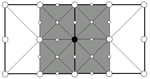
Figure 8. Each edge vertex has four adjacent sub-squares which use it as a corner. If any of those squares are enabled, then the edge vertex must be enabled. For example, the black vertex must be enabled if any of the four gray squares are enabled.
Thus the disable test for an edge vertex becomes straightforward: if the vertex is currently enabled, and the associated reference count is zero, and the vertex test with the current viewpoint returns false, then disable the edge vertex. Otherwise leave it alone. The conditions for disabling a square are fairly straightforward: if the square is currently enabled, and it's not the root of the tree, and none of its edge vertices are enabled, and none of its sub-squares are enabled, and the square fails the box test for the current viewpoint, then disable it.
Memory
A very important issue with this (or any) LOD method is memory consumption. In a fully populated quadtree, a single quadtree square is equivalent to about three vertices of an ordinary heightfield, so it is imperative to keep the square data-structure as compact as possible. Fortunately, the needs of the Update() and Render() algorithms do not require each square to contain all the information about 9 vertices. Instead, this is the laundry list of required data:
5 vertex heights (center, and edges verts east, north, west, south)
6 error values (edge verts east and south, and the 4 child squares)
2 sub-square-enabled reference counts (for east and south verts)
8 1-bit enabled flags (for each edge vertex and each child square)
4 child-square pointers
2 height values for min/max vertical extent
1 1-bit 'static' flag, to mark nodes that can't be deleted
Depending on the needs of the application, the height values can usually be squeezed comfortably into 8 or 16 bits. The error values can use the same precision, or you can also do some non-linear mapping voodoo to squeeze them into smaller data sizes. The reference counts can fit into one byte along with the static flag. The enabled flags fit in one byte. The size of the child-square pointers depends on the maximum number of nodes you anticipate. I typically see node counts in the hundreds of thousands, so I would say 20 bits each as a minimum. The min/max vertical values can be squeezed in various ways if desired, but 8 bits each seems like a reasonable minimum. All told, this amounts to at least 191 bits (24 bytes) per square assuming 8-bit height values. 16-bit height values bring the total to at least 29 bytes. A 32-byte sizeof(square) seems like a good target for a thrifty implementation. 36 bytes is what I currently live with in Soul Ride, because I haven't gotten around to trying to bit-pack the child pointers. Another byte-saving trick I use in Soul Ride is to use a fixed-pool allocator replacement for quadquare::new() and delete(). You can eliminate whatever overhead the C++ library imposes (at least 4 bytes I would expect) in favor of a single allocated bit per square.
There are various compression schemes and tricks that could be used to squeeze the data even smaller, at the expense of complexity and performance degradation. In any case, 36 bytes per 3 vertices is not entirely unrespectable. That's 12 bytes/vertex. [1] reports implementations as small as 6 bytes per vertex. [2] only requires storage of vertex heights and "wedgie thicknesses", so the base data could be quite tiny by comparison. [4], using a modified [2], reports the storage of wedgie thicknesses at a fraction of the resolution of the height mesh, giving further savings.
However, such comparisons are put in a different light when you consider that the quadtree data structure is completely adaptive: in very smooth areas or areas where the viewer won't ever go near, you need only store sparse data. At the same time, in areas of high importance to the game, you can include very detailed features; for example the roadway in a driving game can have shapely speed bumps and potholes.
Geomorphs
[2] and [3] go into some detail on "vertex morphing", or "geomorphs". Basically, geomorphing is a technique whereby when vertices are enabled, they smoothly animate from their interpolated position to their correct position. It looks great and eliminates unsightly popping; see McNally's TreadMarks for a nice example.
Unfortunately, doing geomorphs requires storing yet another height value for the vertices that must morph, which would present a real data-size problem for the adaptive quadtree algorithm as I've implemented it. It could result in adding several bytes per square to the storage requirements, which should not be done lightly. [3] incurs the same per-vertex storage penalty, but [2] avoids it because it only has to store the extra height values for vertices that are actually in the current mesh, not for every vertex in the dataset.
I have three suggestions for how to address the geomorph issue. The first alternative is to spend the extra memory. The second alternative is to optimize the implementation, so that really small error tolerances would be practical and geomorphs unnecessary. Moore's Law may take care of this fairly soon without any additional software work. The third alternative is to split the quadtree into two trees, a "storage tree" and a "mesh tree". The storage tree would hold all the heightfield information and precomputed errors, but none of the transitory rendering data like enabled flags, reference counts, geomorph heights, etc. The mesh tree would hold all that stuff, along with links into the storage tree to facilitate expanding the mesh tree and accessing the height data. The mesh tree could be relatively laissez-faire about memory consumption, because its size would only be proportional to the amount of currently-rendered detail. Whereas the storage tree, because it would be static, could trim some fat by eliminating most of the child links.
The storage-tree/mesh-tree split could also, in addition to reducing total storage, increase data locality and improve the algorithm's cache usage.
Working Code
The Soul Rider engine is closed source for the forseeable future, but I did re-implement the essentials of this algorithm as a companion demo for this article. The demo source is freely available for you to examine, experiment with, and modify and incorporate into your own commercial or non-commercial projects. I only ask that if you do incorporate the demo source into a project, please acknowledge me in the credits!
I didn't sweat the data-packing issue in the demo code. That would be a good area to experiment with. Also, I didn't implement frustum culling of squares, but all the necessary data is readily available.
The data included with the demo comes from USGS 7.5-minute DEMs of the Grand Canyon (USGS). At Slingshot we have a proprietary tool that crunches the USGS data and stitches neighboring DEMs together; I collected 36 datasets and resampled them at a lower resolution to make the heightfield. I made the texture in a few minutes in Photoshop, by loading an 8-bits per sample version of the heightfield as raw data, running the Emboss filter on it to create shading, and adding some noise and tinting. The texture is just one big 1024x1024 image, stretched over the entire terrain.
The data-loading code should be fairly self explanatory, so if you have some of your own data you want to try, it should be easy to get it in there.
The program uses OpenGL and GLUT for 3D, window setup, and input. I developed it under Win98 using a TNT2 card, but I tried to avoid Windows-isms so it should be easy to port to other systems that support GLUT.
Exercises for the Reader
In addition to the tighter data packing I mentioned, there are a few other things in the Soul Ride engine which aren't in the article demo. The big one is a unique-full-surface texturing system, the details of which are beyond the scope of this article. But I will mention that good multi-resolution texturing, especially containing lighting, is extremely beneficial for exploiting the unique features of the quadtree terrain algorithm.
One thing I haven't yet experimented with, but looking at the demo code would be fairly easy to hack in, is on-demand procedural detail. In my view, on-demand procedural detail looms large in the future of computer graphics. There just doesn't seem to be any other good way to store and model virtual worlds to the detail and extent where they really have the visual richness of the real world. Fortunately, the problem is completely tractable, if complicated. I think this quadtree algorithm, because of its scalability, can be helpful to other programmers working on on-demand procedural detail.
Yet another cool extension would be demand-paging of tree subsections. It actually doesn't seem too difficult; basically you'd flag certain quadsquares at any desired spot in the hierarchy as being "special"; they'd contain links to a whole giant sub-tree stored on disk, with the max-error for the sub-tree precomputed and stored in the regular tree. Whenever Update() would try to enable a "special" square, it would actually go off and load the sub-tree and link it in before continuing. Getting it to all stream in in the background without hitching would be a little interesting, but I I think doable. It would result in basically an infinite paging framework. On-demand procedural detail could exploit the same basic idea; instead of chugging the disk drive to get pre-made data, you'd run a terrain-generation algorithm to make the data on the fly.
And another suggestion for further work would be to identifying and eliminating performance bottlenecks. I suspect that there's some headroom in the code for making better use of the graphics API interface.
Acknowledgements
In addition to the authors of the papers (listed below under References) which this work is based on, I would also like to send shout-outs to Jonathan Blow, Seumas McNally and Ben Discoe for their various thought-provoking emails and comments, and also to the participants in the algorithms@3dgamedev.com mailing list, where I've learned a lot of extremely interesting stuff from other programmers about different approaches and the ins-and-outs of terrain rendering.
References
[1] Peter Lindstrom, David Koller, William Ribarsky, Larry F. Hodges, Nick Faust and Gregory A. Turner. "Real-Time, Continuous Level of Detail Rendering of Height Fields". In SIGGRAPH 96 Conference Proceedings, pp. 109-118, Aug 1996.
[2] Mark Duchaineau, Murray Wolinski, David E. Sigeti, Mark C. Miller, Charles Aldrich and Mark B. Mineev-Weinstein. "ROAMing Terrain: Real-time, Optimally Adapting Meshes." Proceedings of the Conference on Visualization '97, pp. 81-88, Oct 1997.
[3] Stefan Röttger, Wolfgang Heidrich, Philipp Slusallek, Hans-Peter Seidel. Real-Time Generation of Continuous Levels of Detail for Height Fields. Technical Report 13/1997, Universität Erlangen-Nürnberg.
[4] Seumas McNally. http://www.LongbowDigitalArts.com/seumas/progbintri.html . This is a good practical introduction to Binary Triangle Trees from [2]. Also see http://www.TreadMarks.com , a game which uses methods from [2].
[5] Ben Discoe, http://www.vterrain.org . This web site is an excellent survey of algorithms, implementations, tools and techniques related to terrain rendering.