Reservoir Computing Toolbox Manual
Автор: Benjamin Schrauwen, David Verstraeten and Michiel D’Haene
Автор: Benjamin Schrauwen, David Verstraeten and Michiel D’Haene
This document describes the Reservoir Computing Toolbox (RCT), a Matlab toolbox that offers a set of functions and scripts to facilitate experiments with Reservoir Computing systems.
Reservoir Computing (RC) is a concept in the field of machine learning that was introduced independently in three similar descriptions: the Liquid State Machine [1], Echo State Networks [2] and the Backpropagation-Decorrelation learning rule [3]. However, each of these ideas share a common basic assumption: a recurrent network of nodes (the reservoir ) with weighted connections is constructed in the beginning of an experiment, and generally left unchanged (except when using reservoir adaptation, see Section 1.5). Instead, a separate classification or regression function (the readout function), is trained on the response of the reservoir to the input signals.
The concepts behind Reservoir Computing are similar to ideas from both kernel methods [4] and recurrent neural network theory. Indeed: much like a kernel, the reservoir projects the input signals into a higher dimensional space (in this case the state space of the reservoir), where a linear regression can be performed. However, there are two major differences between reservoirs and kernel methods. For kernels, there exists a mathematical nicety called the kernel trick, which removes the need to explicitly calculate the projection of the input by the kernel, generally resulting in better computational efficiency. On the other hand, the reservoir - due to the recurrent delayed connections inside the network - has a form of (short) term memory, called the fading memory [5] or the echo state property [2], which allows temporal information contained in the input to be remembered by the reservoir for a theoretically infinite time.
The main advantages of Reservoir Computing are its elegance and simplicity of use. When solving an offline problem using reservoirs, one constructs a random network with a certain topology, simulates it on the training data, and derives a linear classifier that performs optimally on the training set. The latter is usually done using the pseudo-inverse method, which is computationally very efficient and minimizes the squared error on the training set.
This toolbox consists of functions that allow the user to easily set up datasets, reservoir topologies, experiment parameters and to easily process results of experiments. We publish the code as an open source effort under a GPL license, but we strongly encourage contributions from other researchers. It is our hope that the use of a single toolbox that was collectively built and used by the community will speed up and facilitate future research. By using the same codebase, the reproduction and extension of previous research results is far easier. Therefore, if you have extended the functionality of the toolbox for experimentation or research, please send us your code so that we may include it.
Note that the toolbox uses some advanced Matlab features such as structs, function pointers and anonymous functions. To fully understand and use the features of the toolbox or to write your own code, it is advised to read up on these topics in the Matlab documentation.
While the toolbox is essentially that, a box of tools with which to build your own experiments, the directory examples/framework contains a set of scripts that allows the user to conduct large-scale parameter searches for a certain task. This script also showcases a lot of the functionality contained in the toolbox, and as such it can be quite instructive to study this code.
The main simulation flow of the framework is depicted in Figure 1.1.
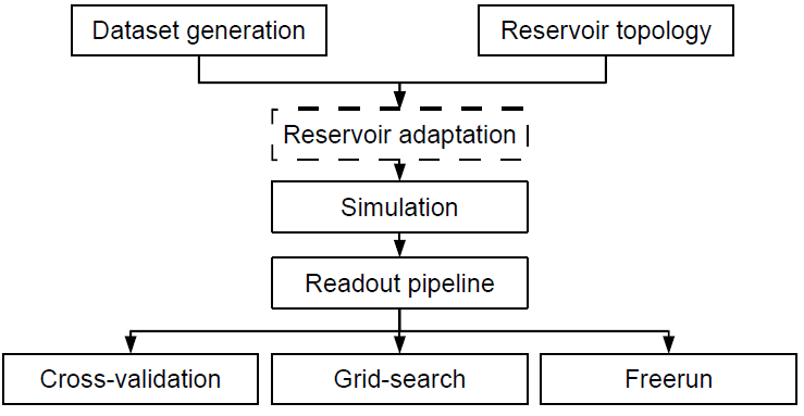
Figure 1.1: Schematic overview of the rc simulate job.m script.
Generally, one experiment or job (which is done by executing rc simulate job.m) will consist of the construction (or loading) of a dataset, and the construction of a reservoir of a given topology. Optionally, the reservoir will be pre-adapted to the dataset using reservoir adaptation (see section 1.5). Next, the actual simulation of the reservoir is done, and the reservoir responses are all saved. Afterwards, a readout function is trained and the performance of the reservoir is evaluated using one of three methodologies: cross-validation (section 1.8.1), grid search (section 1.8.2) or freerun (section 1.8.3).
The rc simulate script has some automation built into it that allows the above flow to be repeated any number of times for any parameter setting. The directory examples/framework contains the file defaults.m with some default settings which will run a basic experiment. To define your own experimental setup and parameters, you can set the variable custom configuration to the name of your script containing the settings, which will be called after defaults.m. Besides all global parameters that remain constant during all runs of one experiment, there is also a special variable parameter ranges, which is a struct array containing two fields, name and range. Here, every parameter can be associated with a range of values across which the rc simulate.m script will loop, and if multiple ranged variables are defined all possible combinations will be visited and simulated. Generally, due to the randomness of the reservoir construction, one will want to simulate every parameter setting a number of times to get a statistically relevant result. This can be done by setting the variable runs.
The toolbox contains a number of standard benchmarks that have been described in literature, and also some other as yet unpublished datasets. The input generation step will create the dataset that will be used to evaluate the reservoir. It should return a Matlab struct array containing at least fields outputs and reservoir (this last field is empty and will be filled in by the reservoir simulation function), and optionally the inputs field. The fields are cell arrays, whereby each cell contains the input or output signals for a single sample in the dataset. The number of input channels and output channels is determined by the first dimension of each cell in the inputs and outputs fields. The second dimension (the number of columns) should be the number of timesteps of each dataset example (for classification tasks, however, each output cell can be a vector with the desired class outputs, which will internally be expanded to a timeseries with constant values). See the .m files contained in the directory dataset generationfor some examples of the types of tasks can be used in the toolbox.
One of the very important parameters that determine the behaviour and performance of an RC system is the topology of the different components. In the RC Toolbox, the topology of the system is completely defined by the topology structure. This structure can be depicted graphically as a single large matrix (see figure 1.2). As the figure shows, the toolbox allows to connect inputs, reservoir and outputs on the one hand to reservoir and outputs on the other hand. The user is free to fill in the components he wants to achieve different setups, with the exception of the reservoir to output connections - these are trained based on the dataset. In the simplest cases, only input to reservoir, reservoir to reservoir and reservoir to output connections exist. This basic setup can be extended in numerous ways, for example:
To fill in these matrices, the toolbox implements a number of functions that can be combined in a pipelined modular manner, whereby the parts of the matrix are fed from function to function to get the desired topology. The first step is to specify which neurons are connected to each other. This is done by setting the relevant positions in the connection matrix to one or zero. Next, an optional rewiring function can be applied, which will take the unweighted connection matrix and rewire certain connections according to a certain method and with a specified probability. Next, the weigths are assigned to the nonzero connections, usually according to some random continuous distribution or chosen randomly from a discrete set. Finally, the whole matrix can be rescaled, either by a constant factor or by setting some global parameter like the spectral radius to a certain value.
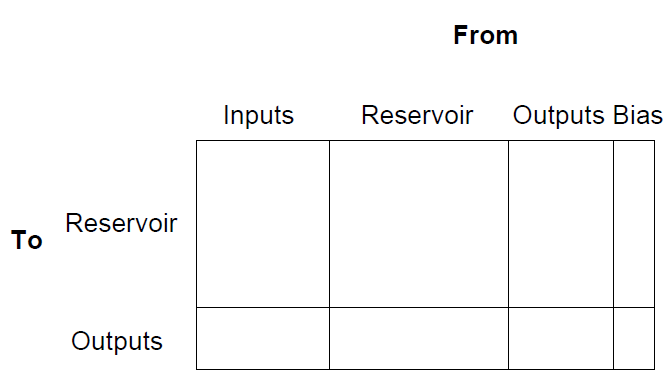
Figure 1.2: The general topology matrix for the RC system.
Before simulating the reservoir on the selected dataset, the user can optionally do reservoir adaptation. In this version, both exponential intrinsic plasticity (applicable to fermi-type activation functions)[6], [7] and gaussian intrinsic plasticity (implemented for tanh-activation functions) [?] are included. To turn on this feature, the parameter adapt.epochs should be set to a value larger than zero. The reservoir will be simulated by feeding the input examples contained in the dataset in a random order, and meanwhile adapting certain internal parameters of the reservoir in an unsupervised way, depending on the type of reservoir adaptation. The function that does the adaptation is set in adapt.function, you can write your own reservoir adaptation algorithm and plug it in here. The whole dataset will be fed adapt.epochs times to the reservoir before going over to the actual simulation and training/testing phase.
Once the reservoir topology is set and the weight matrices have been assigned, the reservoir can be simulated on the dataset. Several different node types are described in literature, ranging from simple analog nodes with no nonlinearity to spiking nodes with dynamic synapses. By specifying the topology.node type parameter, the user can choose between analog or spiking nodes. For analog nodes, the model always performs a weighted sum of the input values followed by a nonlinearity. The nonlinearities currently present in the toolbox are : linear, sign, piecewise linear, tanh and fermi. These can be selected, or others can be added, by setting the variable topology.node func to a pointer to the desired nonlinearity function. For spiking nodes, an interface was built with the neural event-based simulator ESSpiNN [8] based on a neural simulator by Olivier Rochel. With this simulator, a number of socalled discrete-event neural models with optional synapse models can be simulated. Also, the synapses can exhibit adaptive behaviour such as dynamic plasticity, Spike Time Dependent Plasticity.
For analog nodes, the toolbox supports the inclusion of node-level integration (sometimes referred to as analog integrator neurons). Here, every neuron has an internal integration factor that feeds some of the neurons state or output back to itself. This has the effect of slowing the dynamics of the reservoir down. The toolbox supports an integration factor both inside and outside the nonlinearity (see figure 1.3)
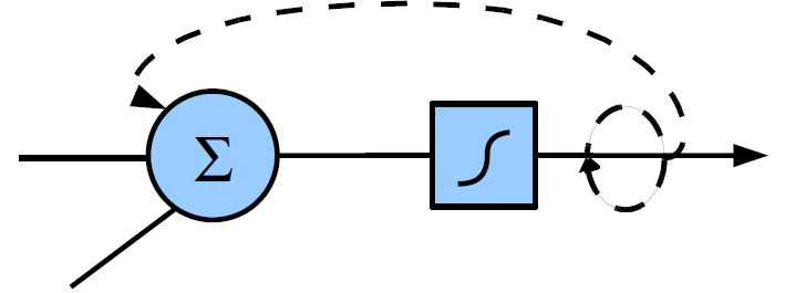
Figure 1.3: Possible types of node integration.
The readout consists of a series of classifiers or regressors, each of which takes the current reservoir state as input and computes a weighted sum. Thus, for every simulated timestep of the reservoir, the readout will give a vector of output values. For certain tasks, however, it is beneficial to post-process this output. For instance, for the recognition of isolated digits, this temporal output of the readout needs to be reduced to a single classification answer. Therefore, the toolbox also implements a readout post-processing pipeline that will apply a series of function to the readout output. The pipeline consists of a spatial transformation (operating at each timestep), followed by a temporal transformation (operating on each regressor), and finally again a spatial transformation. For each of these steps, a number of functions are already present in the toolbox, see the configuration files for examples.
Once the reservoir has been simulated on the dataset, several options exist to evaluate the performance depending on the type of problem and the desired accuracy of the evaluation. The method used to train the readout is set in the parameter train params.train readout. When training the linear readout, regularization is applied through either applying a small amount of gaussian noise to the reservoir responses (when using train pseudo inv, the standard deviation of the noise is set in train params.noise) or by doing ridge regression (when using train ridge readout, the regularization parameter is train params.lambda). Both these regularization parameters can etiher be set by hand in the case of crossvalidation, or optimized using grid-search.
For n-fold cross-validation, the dataset will be split into n chunks. Each of these chunks will separately serve as a testing set, while the rest will serve to train the readout. A common setting for n is 10. The amount of folds is set in the variable train params.folds. If this variable is equal to one, the dataset will be split only once into a training and testing set and the proportion to be used for training needs to be set in train params.opt foldsize - note that this requires less computation but also yields less accurate performance measures since the performance can depend on the selection of training and testing samples.
A more thorough evaluation of the possible performance of one reservoir can be done by using grid-search. Here, a regularization parameter is actively optimized by doing a brute-force grid search of the parameter space. When using train pseudo inv, the regularization noise is optimized, and when using train ridge readout, the λ parameter is optimized. The gridsearch is done hierarchically, by defining an interval across which to search, finding the optimum in that interval, defining a smaller interval around the optimum, and so on. The depth of the hierarchy is set in train params.grid max depth, the number of steps in each interval is train params.regul nrsteps, and the initial interval is [train params.regul min, train params.regul max ]. For each regularization parameter setting, n-fold cross-validation is performed on a separate validation set, and once an optimum is attained, the final performance on an unseen testset is evaluated.
In the case of timeseries generation tasks, the reservoir will be run in freerun mode after training. To enable this, set train params.freerun to true. In this case, the readout will be trained on all samples in the dataset, but only the part up to train params.freerun split. The remainder of each sample is used for testing purposes.
In this case, the input field of the data struct is not mandatory (since it is usually only the teacher-forced output that will be fed back to the reservoir), but it can be set if needed. After the training of the readout, the teacher-forced output is replaced by the actual readout, and the system is left to run on its own. See for instance the mso task under examples for an example.
If the boolean variable save results is set to true, all variables in the workspace are saved to a file after each run. To save disk space, by default the data struct, containing all input, output and reservoir data is deleted before saving the workspace. If these should be saved as well, set the variable save data to true. The files are saved in a subdirectory of the path specified in the variable output directory, and are named with a timestamp. Once the experiment has completed, the toolbox offers some functionality to process the experiment results and to plot the performance results. The function get saved data takes a directory name and a cell array of strings (param names) as input arguments, and will return three arguments, param data, p range and p var. The first argument is a cell array, where each cell contains the values of the variables requested in param names, the second argument contains all the values that particular experiment has ranged over, and the third return argument is a cell array containing the variable names being ranged across. Note that the strings contained in param names are evaluated literally for each of the files, so the user can also request more complex expressions or functions of variables contained in the files. For instance, the line [param data, p range, p var] = get saved data(indir, ’mean(evaluation.train)’, ’mean(evaluation.test)’); will return the mean evaluation training and testing results for each of the files.
By setting the variable do plotting simulation digest to true, the framework will plot some relevant information after each run that allows the user to quickly and informally evaluate the validity of the results. The figure consists of four columns, where the first three contain subplots showing information on two randomly selected samples from the dataset (if there are three or less samples in the dataset, all of them are shown). The top row shows the response of some of the neurons in the reservoir (for clarity, not the full reservoir is plotted). The middle row shows the output of the linear discriminant before the readout pipeline, and the bottom row shows the result for the end of the readout pipeline. In the third column, the top plot shows which of the submatrices in the general topology structure from figure 1.2 are non-zero - these are shown in white. The second row shows a plot of the poles of the reservoir to reservoir connection matrix in the complex plane. These plots do not give a complete picture of the full experiment, so they should only be used to quickly validate wether the results are plausible at all.
If the variable calc lyapunov is set to true, the local lyapunov numbers of the statespace trajectory of the reservoir will be calculated. These numbers offer an approximation of the exponential deviation from a trajectory in a certain point of that trajectory, and as such are a tentative measure for reservoir dynamics. For a detailed discussion on how these numbers are calculated and a discussion of a possible interpretation, see [9]. The values of the local lyapunov numbers are stored in the variables local lyap and local lyap time, where the latter contains the full timeseries of the local lyapunov numbers, and the former is the mean value across the whole trajectory. In order to speed up calculation, these numbers can be calculated in a ‘sampled’ manner, by setting the variable lyap skip to a certain value.
If the variable batch mode is set, the dataset creation and reservoir simulation will be done in a batched manner. The batched simulation mode is used in case of memory problems and should be used in combination with resampling of the input data or reservoir data. When using batched mode, the resampling is done after each batch, so the full data structure is not stored in memory at any point in time. When using batch mode, the dataset generation function should support this also, see for instance dataset analog speech for an example. The dataset will be split up into batches of batch size samples.
When the parameter train params.fisher labeling is set to @fisher labeling multiple or @fisher labeling single, the class labels for multi-class resp. single-class classification problems are weighted by the relative amount of positive examples in the dataset for each class. This has the effect that a linear discriminant trained with the pseudo-inverse method becomes a Fisher linear discriminant [10]. This usually improves results for clasification problems.
1. W. Maass, T. Natschl?ager, and H. Markram. Real-time computing without
stable states: A new framework for neural computation based on perturbations.
Neural Computation, 14(11):2531–2560, 2002.
2. H. Jaeger. The “echo state” approach to analysing and training recurrent neural
networks. Technical Report GMD Report 148, German National Research
Center for Information Technology, 2001.
3. J. J. Steil. Backpropagation-Decorrelation: Online recurrent learning with
O(N) complexity. In Proceedings of IJCNN ’04, volume 1, pages 843–848,
2004.
4. Bernhard Sch?olkopf and Alex J. Smola. Learning with Kernels: Support Vector
Machines, Regularization, Optimization and Beyond. MIT Press, 2002.
5. W. Maass, T. Natschlger, and Markram H. Fading memory and kernel properties
of generic cortical microcircuit models. Journal of Physiology, 98(4-
6):315–330, 2004.
6. Jochen Steil. Online reservoir adaptation by intrinsic plasticity for
backpropagation-decorrelation and echo state learning. Submitted to Neural
Networks: special issue on Reservoir Computing, 2006.
7. J. Triesch. Synergies between intrinsic and synaptic plasticity in individual
model neurons. In Neural Information Processing Systems, volume 17, 2004.
8. M. D’Haene, B. Schrauwen, and D. Stroobandt. Accelerating event based
simulation for multi-synapse spiking neural networks. In Proceedings of the
16th International Conference on Artificial Neural Networks, volume 4131,
pages 760–769, Athens, 9 2006. Springer Berlin / Heidelberg.
9. David Verstraeten, Benjamin Schrauwen, Michiel D’Haene, and Dirk
Stroobandt. A unifying comparison of reservoir computing methods. Neural
Networks, 2006. submitted.
10. R. O. Duda, P. E. Hart, and D. G. Stork. Pattern Classification - Second
Edition. John Wiley and Sons, Inc., 2001.